Validation
On this page, we present numeric experiments for problems for which analytic solutions are known. By such comparison, we can validate the implemented solvers in OpenDiHu.
1D Poisson
We solve the 1D Poisson equation with linear, quadratic and cubic Hermite elements and conduct a convergence study. The resulting linear system of equations is solved directly using LU decomposition. Note that Hermite ansatz is only experimental, while linear and quadratic ansatz functions can safely be used.
Problem definition
The 1D Poisson problem on a finite interval is given by
We use the following right hand side.
We impose Dirichlet boundary conditions at both ends of the interval.
Analytic solution
The following function fulfills the formulated boundary value problem.
Numeric solution
We discretize the 1D domain with linear, quadratic and cubic Hermite elements with a given numbers of elements, \(n\). The following plots show the result for \(n=6\).
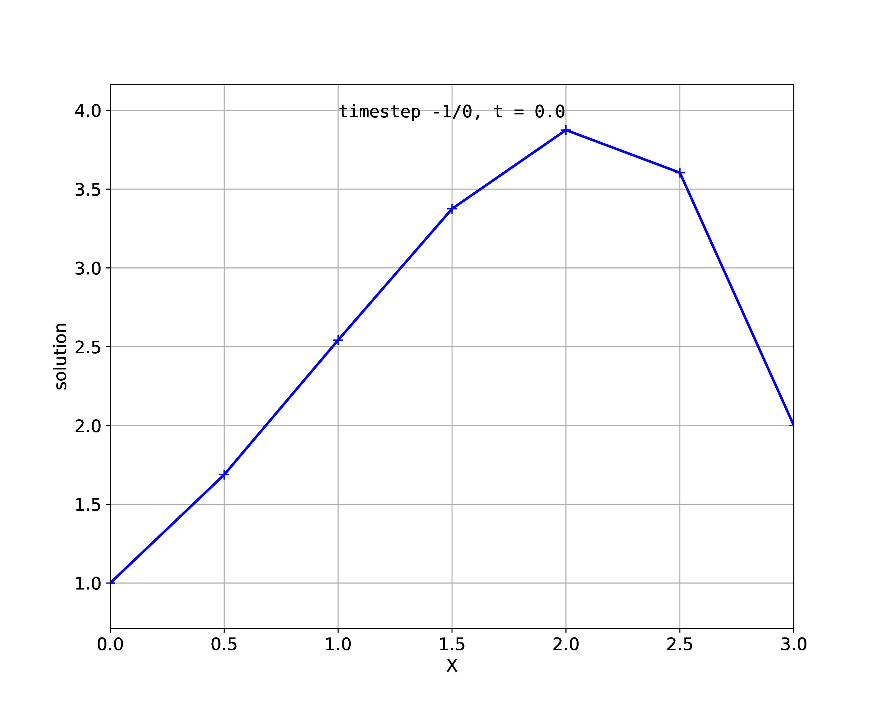
Fig. 81 Numeric solution with 6 linear elements
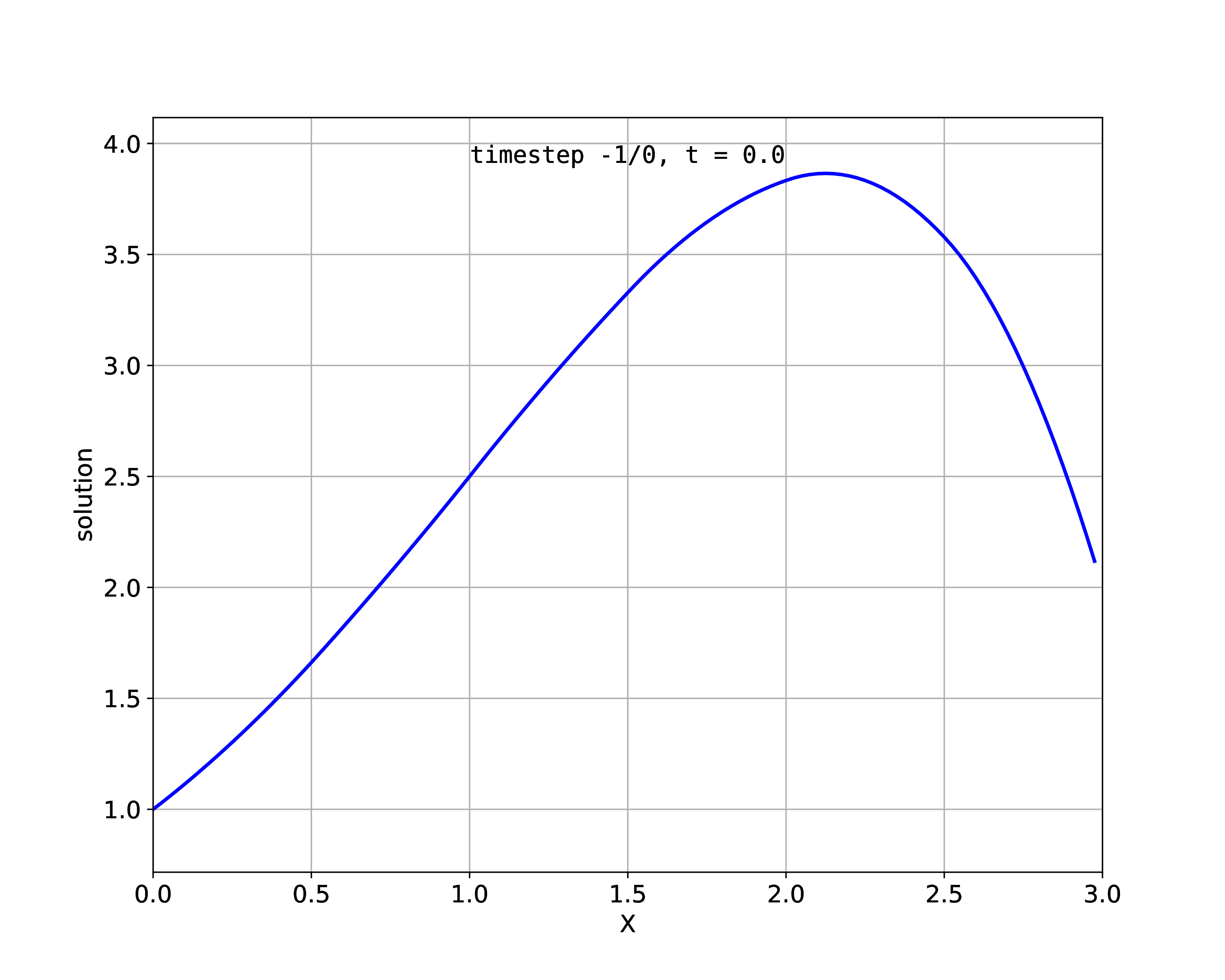
Fig. 82 Numeric solution with 6 quadratic elements
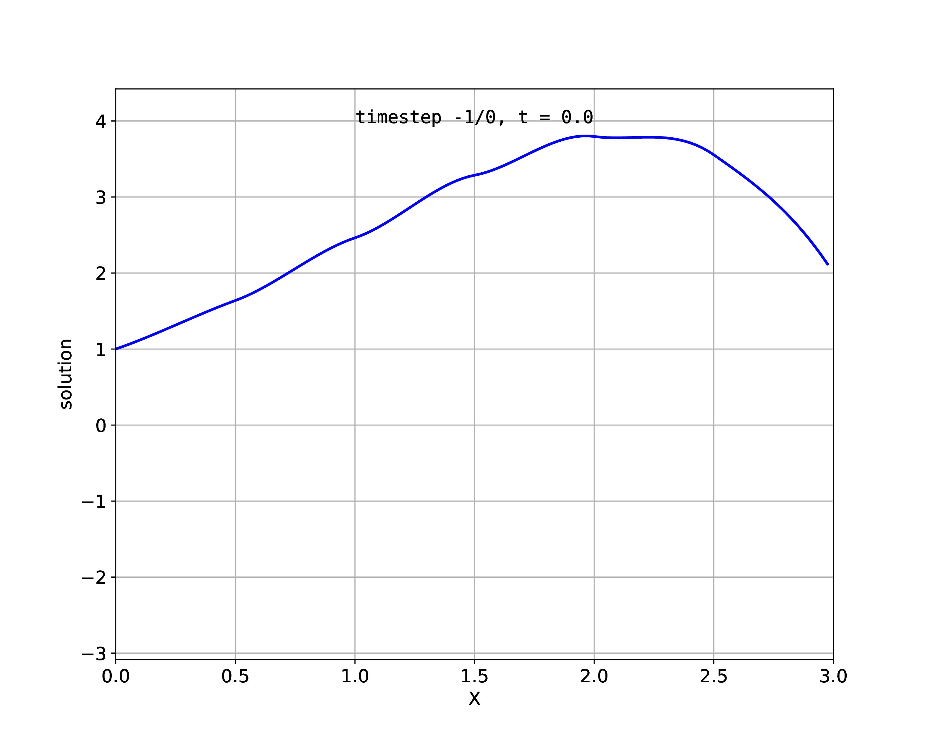
Fig. 83 Numeric solution with 6 Hermite elements
Convergence study
To assess the convergence behaviour, we increase \(n\) from 10 to 100 and compute the \(\mathcal{L}_2\)-error against the analytic solution.
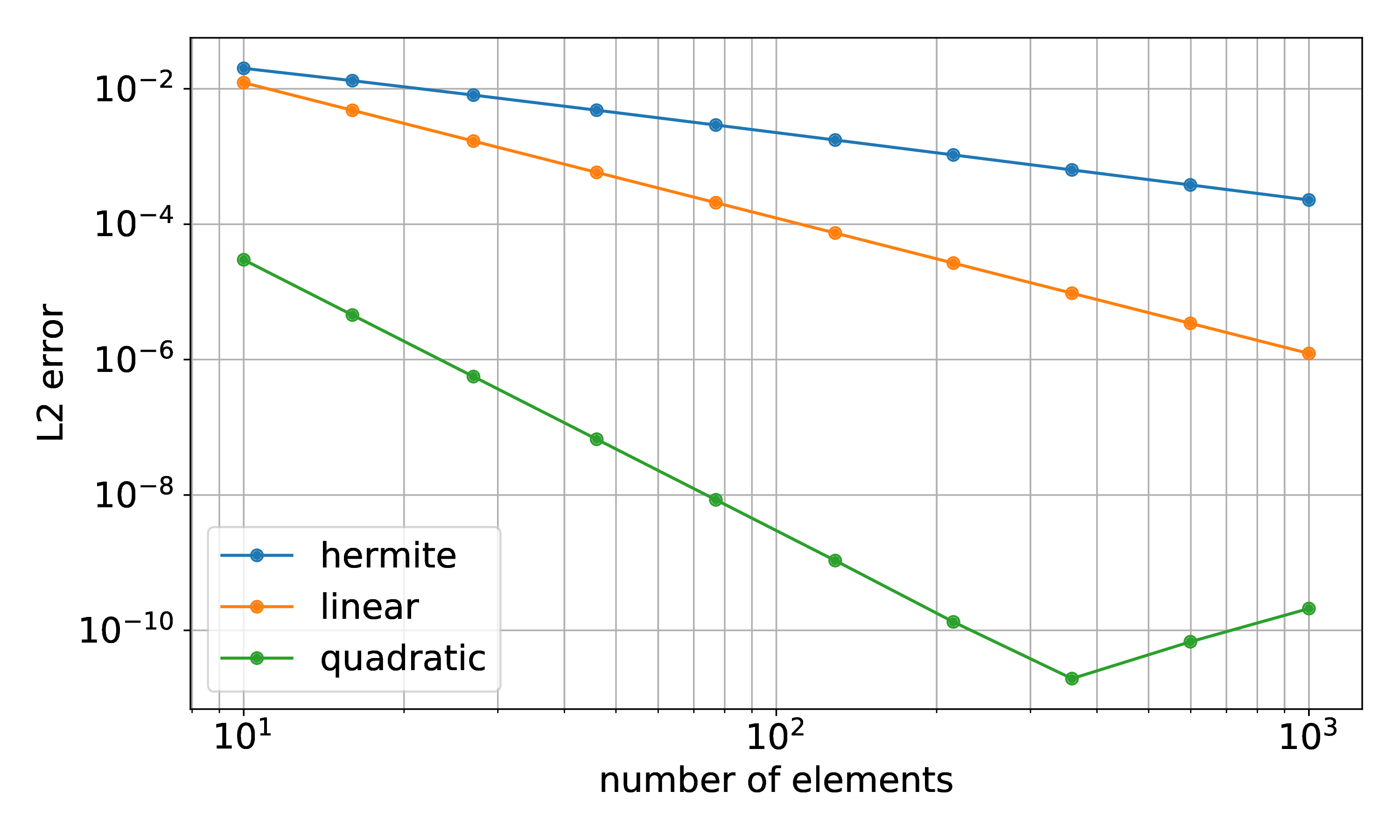
Fig. 84 Result of a convergence study, L2 error against number of elements
The experimental order of converge \(\frac{log(\varepsilon_i)-log(\varepsilon_{i-1})}{log(n_i)-log(n_{i-1})}\) is determined to be as follows.
Linear elements |
-2 |
Quadratic elements |
-4 |
Hermite elements |
-1 |
The linear and quadratic formulations exhibit the expected order of convergence of exactly second order for linear elements and at least third order for quadratic elements. Note that the solution \(u(x)\) has no \(x^3\)-term, therefore the order of convergence is exactly 4 with the quadratic ansatz.
For the quadratic ansatz, the error does not continue to decrease further below \(2^{-11}\) for \(n=600\) elements and more because machine precision is reached in the solver and/or the computation of the L2 error.
The Hermite formulation in OpenDiHu is experimental. The observed convergence order lies around 1. Using Hermite ansatz functions required more effort in the problem specification, because we have to define also boundary conditions for the first derivative \(u'(0)\). In OpenDiHu, using the Hermite ansatz requires specification of both the right hand side function \(f\) and its derivative \(f'\).
How to reproduce
Build the example
cd $OPENDIHU_HOME/examples/validation/poisson_1d
mkorn && sr       # build
Run the simulation for a given number of elements, e.g., 6 elements.
cd $OPENDIHU_HOME/examples/validation/poisson_1d/build_release

./linear ../settings_poisson_1d.py 6
./quadratic ../settings_poisson_1d.py 6
./hermite ../settings_poisson_1d.py 6
Plot the results (make sure that the
$OPENDIHU_HOME/scriptsdirectory is in thePYTHONPATHenvironment variable).cd $OPENDIHU_HOME/examples/validation/poisson_1d/build_release/out plot linear.py plot quadratic.py plot hermite.py # (instead you can also call `plot out/linear.py` etc. from one directory above)
Compute the error for the current simulation results.
cd $OPENDIHU_HOME/examples/validation/poisson_1d
python3 compute_error.py
Conduct the convergence study.
cd $OPENDIHU_HOME/examples/validation/poisson_1d/build_release
python3 ./do_convergence_study.py
3D Poisson
The next validation scenario is a more complex Poisson problem in a 3D domain.
Problem definition
The 1D Poisson problem is given by
We define the following right hand side.
We use the following Dirichlet boundary conditions \(u(\textbf{x}) = \bar{u}(\textbf{x})\) on \(\textbf{x} \in \partial \Omega\)
Analytic solution
The following function fulfills the formulated boundary value problem.
Numeric solution
We discretize the domain \(\Omega = [0, 2] \times [0,3] \times [0,4]\) by
(a) \(\quad 2\,n\times 3\,n \times 4\,n\quad\) linear and quadratic elements, and by
(b) \(\quad n\times n \times n\quad\) linear and quadratic elements.
In case (a), the elements have a cube shape while in (b) they are cuboid shaped with different element lengths along the coordinate axes.
The resulting solution can be seen in the three following plots, for \(n=2\) and \(z=1, z=2\), and \(z=3\).
The resulting \(\mathcal{L}_2\)-errors to the analytic solution are given in Table 3. It can be seen that the error is at machine precision for every tested discretization.
case |
ansatz functions |
number of degrees of freedom |
\(\mathcal{L}_2\)-norm of error |
|---|---|---|---|
(a) |
Linear |
60 |
1.1e-14 |
315 |
8.7e-14 |
||
910 |
1.9e-13 |
||
1989 |
3.7e-13 |
||
(a) |
Quadratic |
315 |
1.7e-13 |
1989 |
6.4e-13 |
||
6175 |
1.3e-12 |
||
14025 |
1.3e-11 |
||
(b) |
Linear |
27 |
2.0e-14 |
125 |
6.9e-14 |
||
512 |
1.7e-13 |
||
1989 |
3.7e-13 |
||
(b) |
Quadratic |
125 |
9.5e-14 |
729 |
3.6e-13 |
||
3375 |
1.8e-12 |
||
12167 |
8.1e-12 |
How to reproduce
Build the example
cd $OPENDIHU_HOME/examples/validation/poisson_3d
mkorn && sr       # build
Run the simulation for a given element number \(n\), e.g. \(n=1\)
cd $OPENDIHU_HOME/examples/validation/poisson_3d/build_release

# case (a) - cube shaped elements
./linear_regular ../settings_poisson_3d.py 1
./quadratic_regular ../settings_poisson_3d.py 1

# case (b) - cuboid shaped elements
./linear_structured ../settings_poisson_3d.py 1
./quadratic_structured ../settings_poisson_3d.py 1
Compute the error for the current simulation results.
cd $OPENDIHU_HOME/examples/validation/poisson_3d
python3 compute_error.py
2D Diffusion
Next, the parabolic diffusion equation with a constant coefficient is used to validate the respective solvers.
Problem definition
The 2D Diffusion problem is formulated as
The diffusion factor is chosen to be constant \(D=3\).
The initial values are given by the following function,
This function describes a peak of height 2 at \(\textbf{p}=(2,5)^\top\). The function decays in radial direction away from \(\textbf{p}\) and reaches constant zero at the boundary \(\partial \Omega\).
We consider two scenarios (a) and (b). In (a), we impose homogeneous Dirichlet boundary conditions at \(x=0\),
In scenario (b) we specify homogeneous Neumann boundary conditions at \(x=0\),
Analytic solution
It is known that a solution to the governing diffusion equation on the 2D infinite domain \(\Omega_\infty = \mathbb{R}^2\) is given by [Ursell2016],
with Green’s Function
For scenario (a) with homogeneous Dirichlet boundary at \(x=0\), we can construct a new function \(G_D\) as sum of \(G(x)\) and its mirrored counterpart \(-G(-x)\) whose graph is mirrored around the \(x=0\) axis,
This function is zero for \(x=0\).
Similarly, for the Neumann boundary in scenario (b), we construct a function
We get an analytic solution for scenario (a) by replacing \(G\) by \(G_D\) in Eq. (1) and for scenario (b) by replacing \(G\) by \(G_N\) in (1). This solution, however, is correct only for a problem on \(\Omega = [0, \infty) \times (-\infty, \infty)\).
Numeric solution
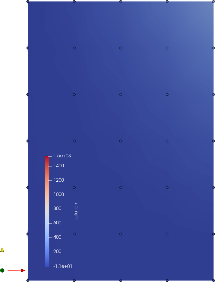
With our finite element solver, we can only discretize a finite domain. The considered problem on \(\Omega = [0,10]\times [0,10]\) with the given initial values is specified such that large changes in function value \(u\) mainly occur in the interior of the domain, away from the boundary at \(x=10, y=0,\) and \(y=10\).
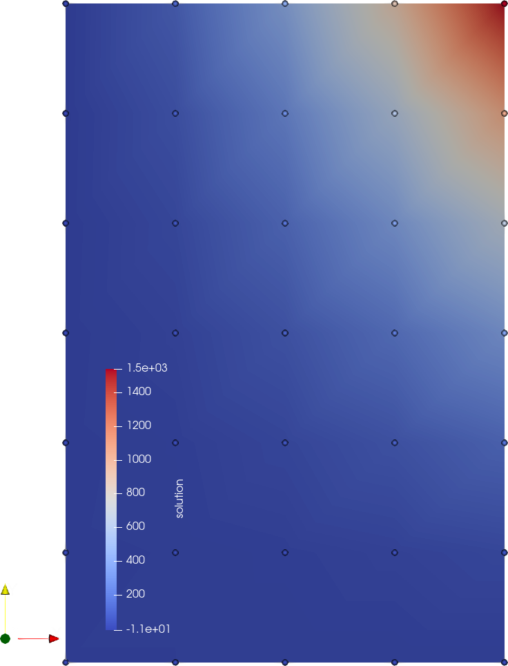
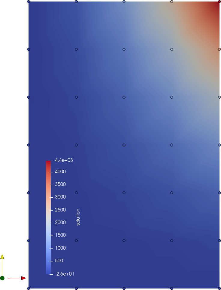
Fig. 85 and Fig. 86 show the initial values \(u(\textbf{x}, 0)\) and the values for \(t=1\), \(u(\textbf{x}, 1)\) for scenarios (a) and (b), respectively.
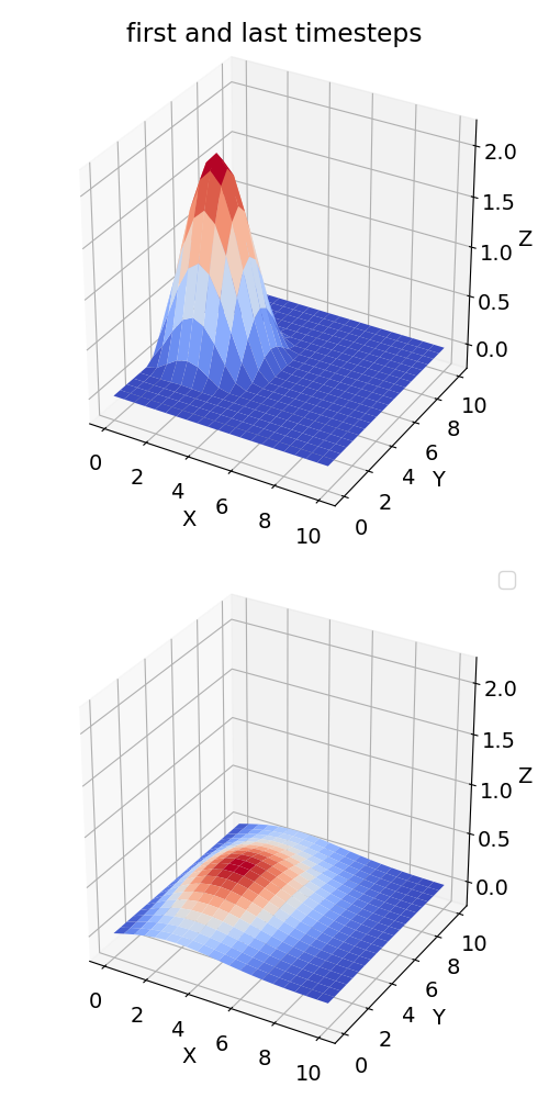
Fig. 85 Scenario (a) with homogeneous Dirichlet boundary conditions at \(x=0\), for \(t=0\) (top) and \(t=1\) (bottom).
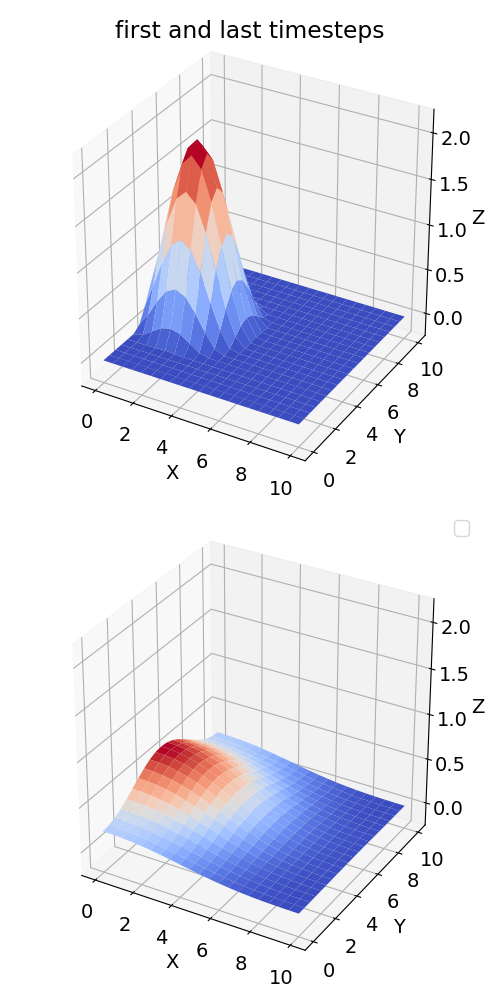
Fig. 86 Scenario (b) with homogeneous Neumann boundary conditions at \(x=0\), for \(t=0\) (top) and \(t=1\) (bottom).
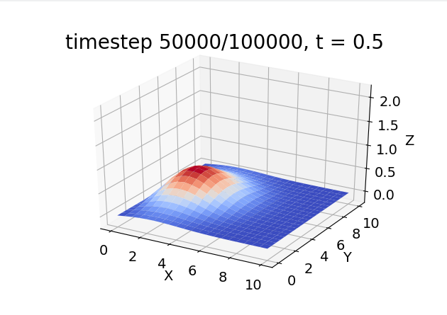
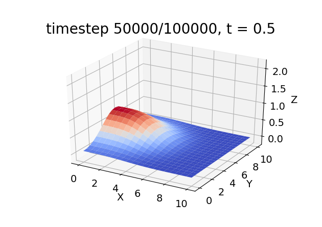
It can also be seen how the different boundary conditions affect the solution value. While the Dirichlet boundary conditions in scenarios (a) absorbs the concentration \(u\) at \(x=0\), the homogeneous Neumann boundary condition serves as a reflection boundary which leads to a constant concentration gradient orthogonal to the wall. The comparison of the state at \(t=0.5\) in the following images (Scenario (a) left, scenario (b) right) shows that concentration decreases faster with the Dirichlet boundary condition.
We disretize the problem in space by \(10\times 10\) quadratic Finite Elements and in time using the Crank-Nicolson scheme with time step width \(dt = 1e-5\). The linear system of equations in every timestep is solved by a geometric multi-grid solver.
Comparison of numeric and analytic solutions
We compare the solution value \(u(\textbf{x},t)\) over time at selected nodes of the Finite Element mesh. The quadratic mesh has \(21 \times 21\) nodes that span the \([0,10] \times [0,10]\) domain. Fig. 87 and Fig. 88 show the results for scenario (a) and scenario (b), the selected nodes are given in the legend.
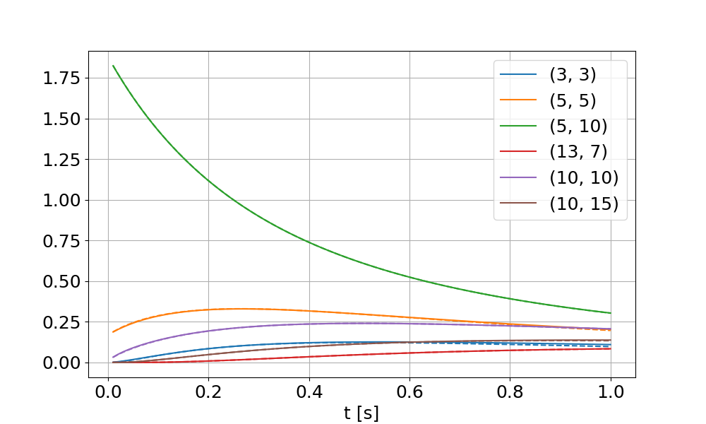
Fig. 87 Scenario (a): Numeric (solid lines) and analytic solution (dashed lines) for selected nodes in the mesh.
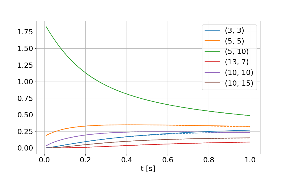
Fig. 88 Scenario (b): Numeric (solid lines) and analytic solution (dashed lines) for selected nodes in the mesh.
It can be seen that the analytic and numeric plots essentially coincide. At some points, the solution starts to differ during the end of the simulation time span, which can be explained by the analytic solution being correct for the infinite domain.
This result shows that the diffusion problem solver of OpenDiHu is validated.
How to reproduce
Build the example
cd $OPENDIHU_HOME/examples/validation/diffusion_2d
mkorn && sr       # build
Run the simulations
cd $OPENDIHU_HOME/examples/validation/diffusion_2d/build_release

# scenario (a)
./diffusion2d_quadratic ../settings_diffusion_2d_dirichlet.py

# scenario (b)
./diffusion2d_quadratic ../settings_diffusion_2d_neumann.py
Visualize the numeric solutions (make sure that the
$OPENDIHU_HOME/scriptsdirectory is in thePYTHONPATHenvironment variable)cd $OPENDIHU_HOME/examples/validation/diffusion_2d/build_release # scenario (a) plot out_dirichlet/* # scenario (b) plot out_neumann/*
Calculate the analytic solution and create the plot
cd $OPENDIHU_HOME/examples/validation/diffusion_2d

# scenario (a)
python3 compute_error_dirichlet.py

# scenario (b)
python3 compute_error_neumann.py
CellML models
We solve CellML models with OpenCOR and OpenDiHu and compare the results. CellML is a description standard for differential-algebraic systems of equations used in the bioengineering community. The XML based CellML file format can be parsed and solved by both OpenCOR and OpenDiHu.
Hodgkin-Huxley (1952)
The most basic electrophysiology model was formulated by Hodgkin and Huxley (1952). It contains four state variables \(V_m\), \(n\), \(h\), \(m\). We set a constant stimulation current of \(i_\text{Stim} = 10 μA/cm^2\) and solve the system for \(t_\text{end}=35 ms\) with Heun’s method and a time step witdh of \(dt=1e-5 ms\).
As a reference, the same simulation is performed with OpenCOR. The resulting values show good agreement.
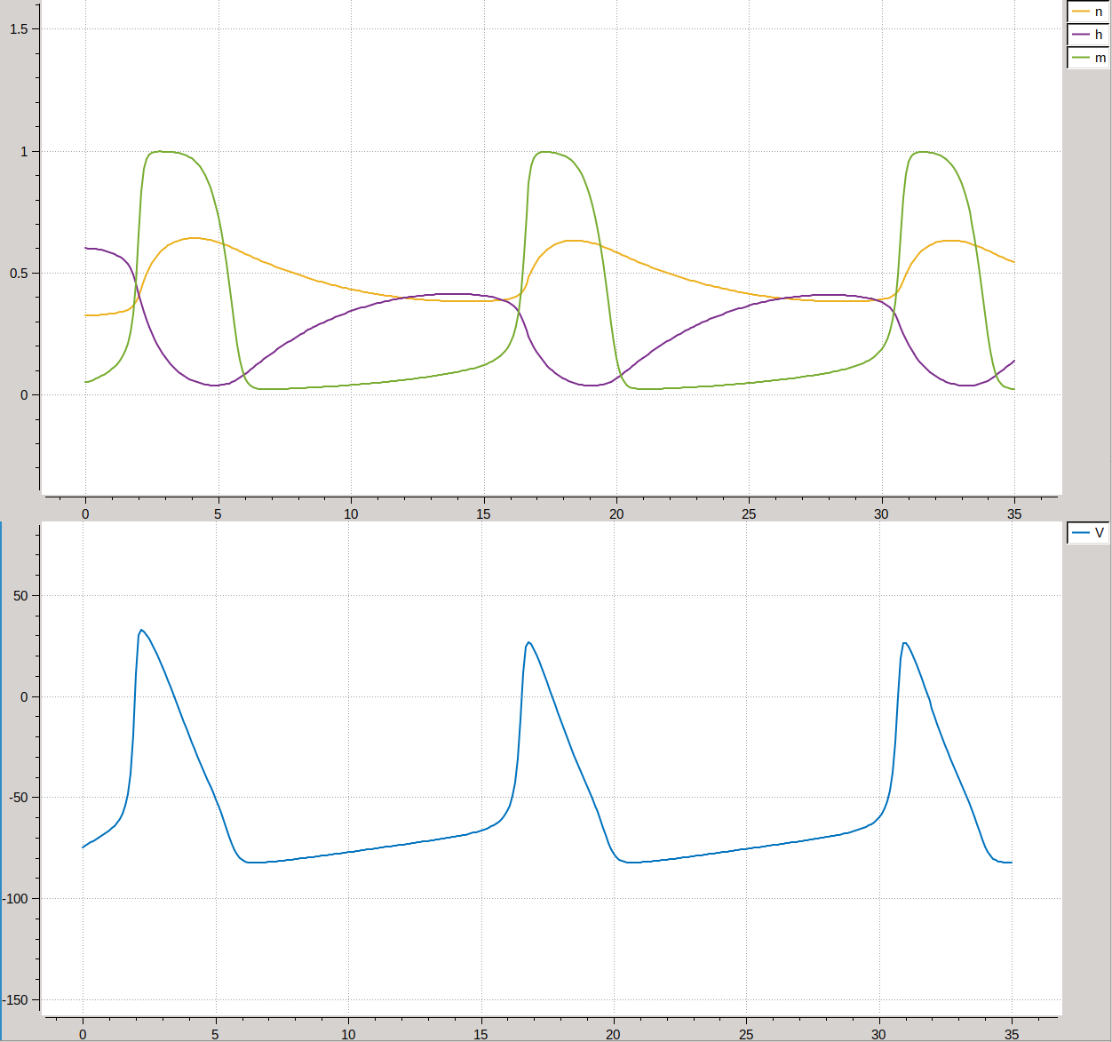
Fig. 89 Visualization of the results in the OpenCOR GUI
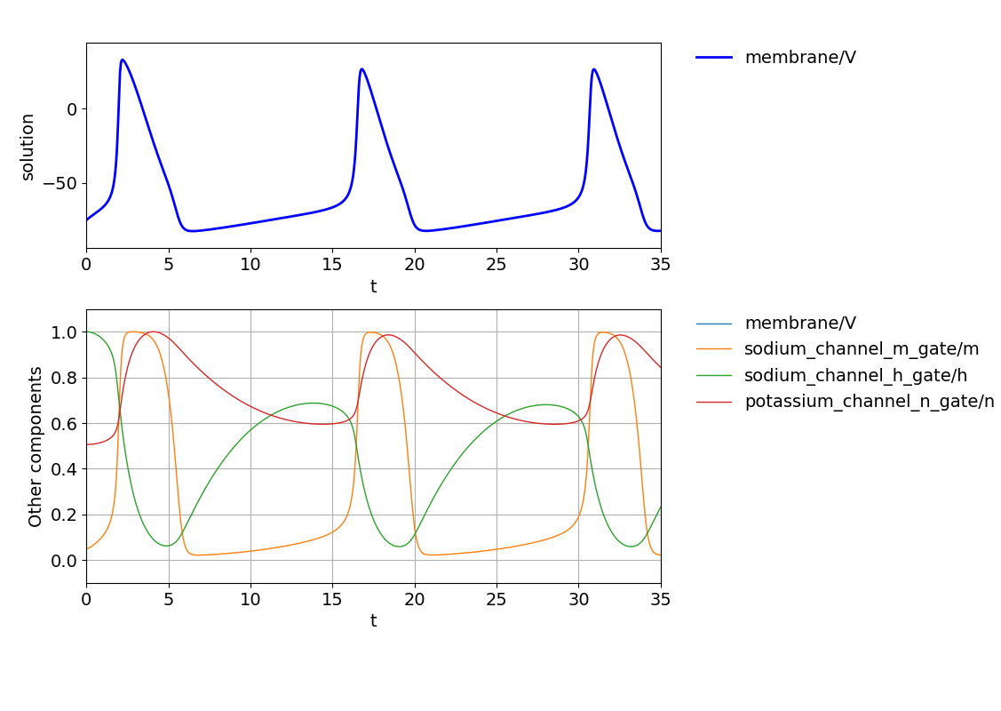
Fig. 90 Visualization of the results from OpenDiHu with the OpenDiHu plot script
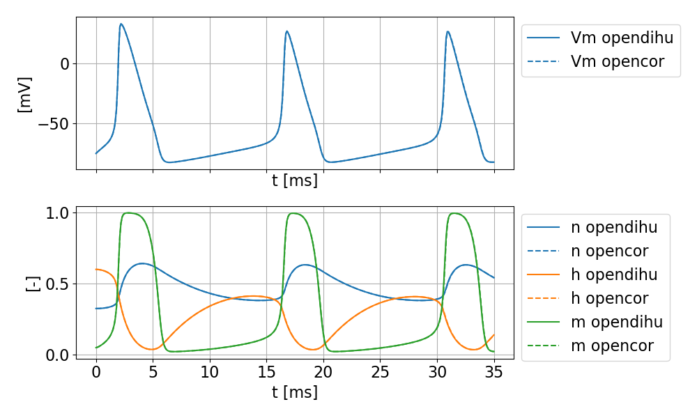
Fig. 91 Comparison of results computed by OpenCOR (dashed lines) and OpenDiHu (solid lines), which show good agreement.
The \(\mathcal{L}_2\)-errors for the solved variables over the entire timespan are given below.
variable |
\(\mathcal{L}_2\)-error |
|---|---|
\(V_m\) |
2.0e-03 |
\(n\) |
3.3e-06 |
\(h\) |
4.2e-06 |
\(m\) |
1.9e-05 |
Shorten, Ocallaghan, Davidson, Soboleva (2007)
Another relevant CellML model is the model by Shorten, Ocallaghan, Davidson, Soboleva (2007).
It consists of 58 ordinary differential equations and 77 algebraic equations that have to be solved in time.
We repeat the previous study with this model using the same numerical parameters and present the result in the following.
The stimulation current wal_environment/I_HH is set to 50.
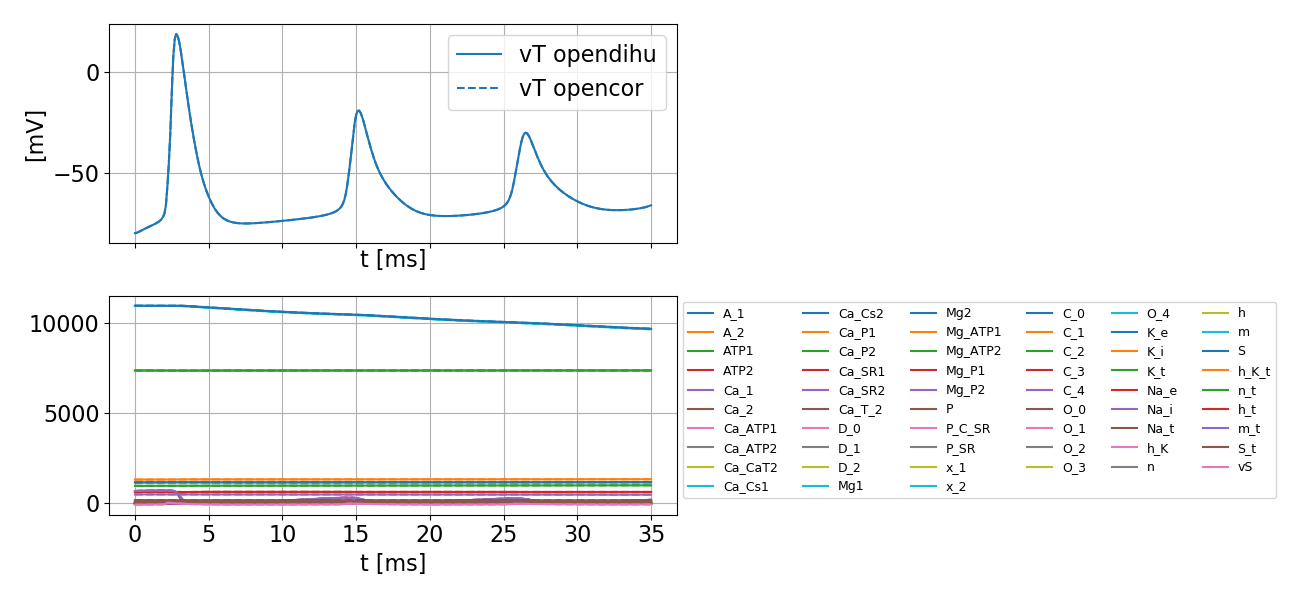
Fig. 92 Comparison of results computed by OpenCOR (dashed lines) and OpenDiHu (solid lines), which show good agreement.
The \(\mathcal{L}_2\)-errors over all timesteps for all state variables are given below. It can be seen that they show good agreement with the reference simulation.
variable |
\(\mathcal{L}_2\)-error |
variable |
\(\mathcal{L}_2\)-error |
variable |
\(\mathcal{L}_2\)-error |
variable |
\(\mathcal{L}_2\)-error |
|---|---|---|---|---|---|---|---|
A_1 |
5.7e-06 |
A_2 |
3.5e-06 |
ATP1 |
1.3e-03 |
ATP2 |
3.6e-04 |
Ca_1 |
9.9e-04 |
Ca_2 |
1.1e-04 |
Ca_ATP1 |
1.4e-03 |
Ca_ATP2 |
3.7e-04 |
Ca_CaT2 |
2.5e+01 |
Ca_Cs1 |
2.6e-02 |
Ca_Cs2 |
2.7e-02 |
Ca_P1 |
2.9e-03 |
Ca_P2 |
3.3e-04 |
Ca_SR1 |
1.8e-02 |
Ca_SR2 |
1.8e-02 |
Ca_T_2 |
2.5e+01 |
D_0 |
9.2e-06 |
D_1 |
1.9e-05 |
D_2 |
5.7e-05 |
Mg1 |
2.9e-03 |
Mg2 |
2.8e-03 |
Mg_ATP1 |
2.9e-03 |
Mg_ATP2 |
2.8e-03 |
Mg_P1 |
2.8e-04 |
Mg_P2 |
2.9e-04 |
P |
2.9e-06 |
P_C_SR |
2.9e-07 |
P_SR |
2.9e-08 |
x_1 |
0.0e+00 |
x_2 |
0.0e+00 |
C_0 |
1.9e-05 |
C_1 |
1.3e-05 |
C_2 |
5.9e-06 |
C_3 |
8.1e-07 |
C_4 |
3.2e-08 |
O_0 |
3.8e-11 |
O_1 |
6.3e-10 |
O_2 |
7.3e-09 |
O_3 |
2.5e-08 |
O_4 |
2.2e-08 |
K_e |
3.0e-06 |
K_i |
2.8e-04 |
K_t |
1.3e-05 |
Na_e |
3.2e-04 |
Na_i |
2.7e-05 |
Na_t |
2.8e-04 |
h_K |
3.3e-07 |
n |
1.6e-05 |
h |
8.2e-06 |
m |
8.1e-05 |
S |
3.0e-07 |
h_K_t |
6.1e-05 |
n_t |
1.5e-05 |
h_t |
1.3e-05 |
m_t |
8.2e-05 |
S_t |
2.8e-07 |
vS |
5.2e-03 |
vT |
4.4e-03 |
How to reproduce
Build the example
cd $OPENDIHU_HOME/examples/validation/cellml
mkorn && sr       # build
Run the simulations
cd $OPENDIHU_HOME/examples/validation/cellml/build_release

./hodgkin_huxley ../settings_cellml.py
./shorten ../settings_cellml.py
Visualize the numeric solutions (make sure that the
$OPENDIHU_HOME/scriptsdirectory is in thePYTHONPATHenvironment variable)cd $OPENDIHU_HOME/examples/validation/cellml/build_release plot out_hodgkin_huxley/* plot out_shorten/*
Compute the L2 errors and generate the comparison plot
The reference values were simulated in OpenCOR (set
wal_environment/I_HHmanually to 50) and then exported as csv files, only selected the state variables to be included in the file. The repository contains these reference values in the directory$OPENDIHU_HOME/examples/validation/cellml/in the fileshodgkin_huxley_1952_data_istim10_opencor.csvandshorten_ocallaghan_davidson_soboleva_2007_no_stim_data_ihh50_opencor.csv.cd $OPENDIHU_HOME/examples/validation/cellml python3 compute_error_hodgkin_huxley.py python3 compute_error_shorten.py
Nonlinear solid mechanics
To validate the implementation of the nonlinear incompressible solid mechanics solver, a comparison against results from the FEBio solver are conducted. Two test case of a tensile test and a shear test are simulated with both solvers. Three different formulations of incompressible hyperelasticity in OpenDiHu are compared with the reference solution from FEBio and found to be equal.
The description of the setup and the results can be found in the dissertation, chapter 8.2.2 [Maier2021].
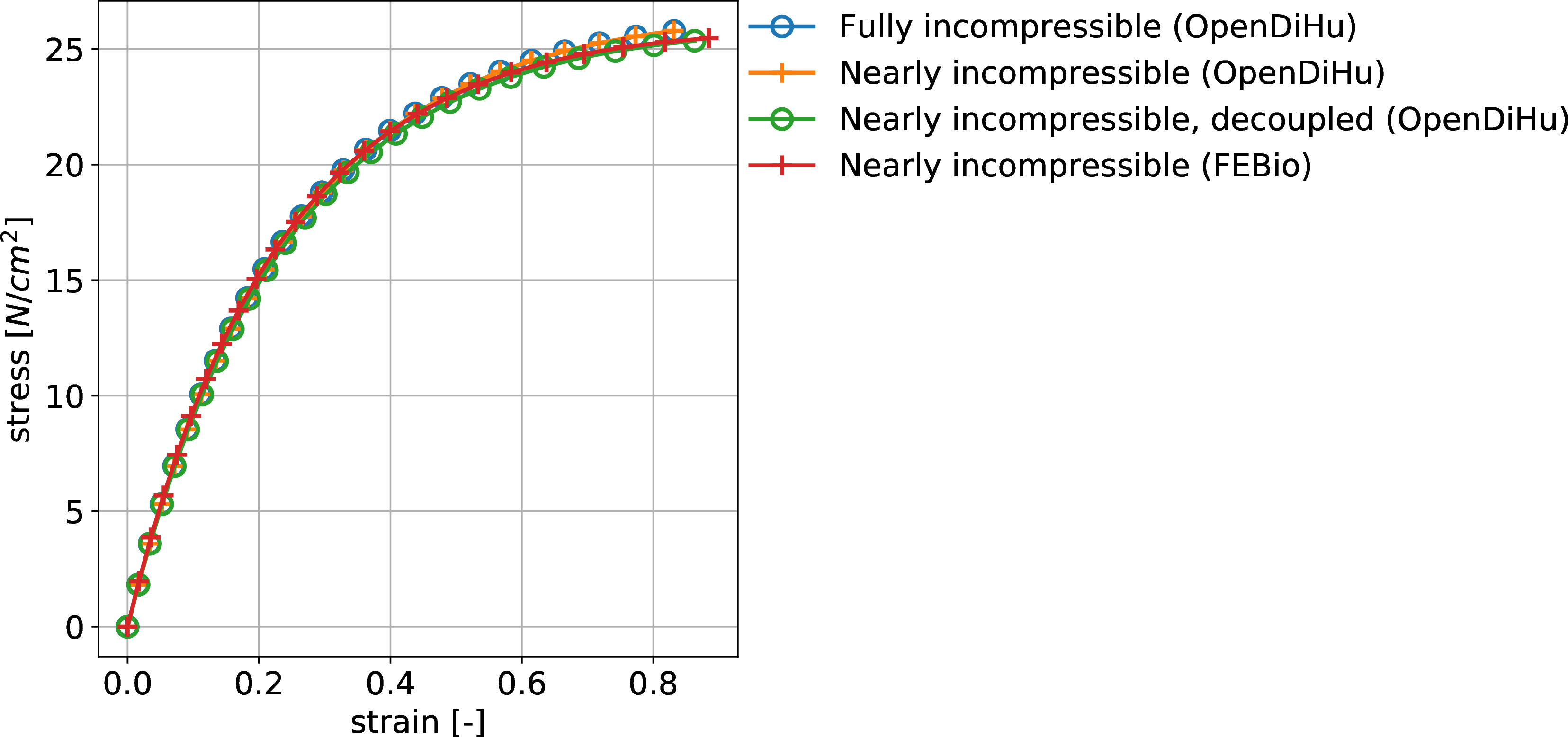
Fig. 93 Resulting stresses in the tensile test showing good match between the different formulations with OpenDiHu and the reference solver FEBio
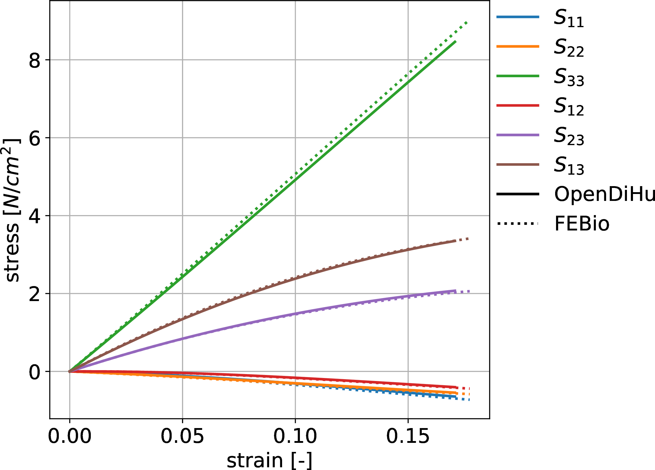
Fig. 94 Resulting stress components in the shear test with good match to the reference solver FEBio
Maier (2021), Scalable Biophysical Simulations of the Neuromuscular System, Ph.D. thesis, University of Stuttgart, 2021
How to reproduce
Build the example
# tensile test
cd $OPENDIHU_HOME/opendihu/examples/solid_mechanics/tensile_test
mkorn && sr

# shear test
cd $OPENDIHU_HOME/opendihu/examples/solid_mechanics/shear_test
mkorn && sr
Run the simulations
For the FEBio simulations to work you need FEBio 3 installed (such that it can be called from the command line as
febio3). If FEBio is not installed, the OpenDiHu simulations will still run, but the reference data will not be available in the plot.# tensile test cd $OPENDIHU_HOME/examples/solid_mechanics/tensile_test/build_release ../run_force.sh # shear test cd $OPENDIHU_HOME/examples/solid_mechanics/shear_test/build_release ../run_force.sh
Visualize the results
# tensile test
cd $OPENDIHU_HOME/examples/solid_mechanics/tensile_test
python3 plot_validation.py

# shear test
cd $OPENDIHU_HOME/examples/solid_mechanics/shear_test
python3 plot_validation.py
Excited cuboid muscle
For more complex multi-scale models, no analytic solutions are available and a direct verification of the solver becomes impossible. A qualitative validation can be carried out by comparing to other groups simulation. In the following, we compute a scenario similar to the one in [Heidlauf2016], chapter 7.3.1.
A cuboid muscle of size \(2.9 \times 1.2 \times 6\) cm has \(31 \times 13\) embedded muscle fibers. The fibers are organized in 10 motor units which are activated from a motor neuron model, as described in [Heidlauf2016]. We use the same discharge times as the author. We the discretize the fibers by 145 linear Finite Elements as in [Heidlauf2016]. No information is given about the 3D domain discretization, for which we use \(15 \times 5 \times 33 = 2475\) quadratic Finite Elements. A difference between our simulation and the one in [Heidlauf2016] is that we omit the fat layer and use a more realistic dynamic solid mechanics formulation instead of the quasi-static formulation.
The contraction state in our simulation is shown below and can be compared to Fig. 7.4 in [Heidlauf2016]. (Note that we set the “displacementsScalingFactor” to 5, equal to the visualization in the referenced thesis.) The contraction shows qualitative agreement.
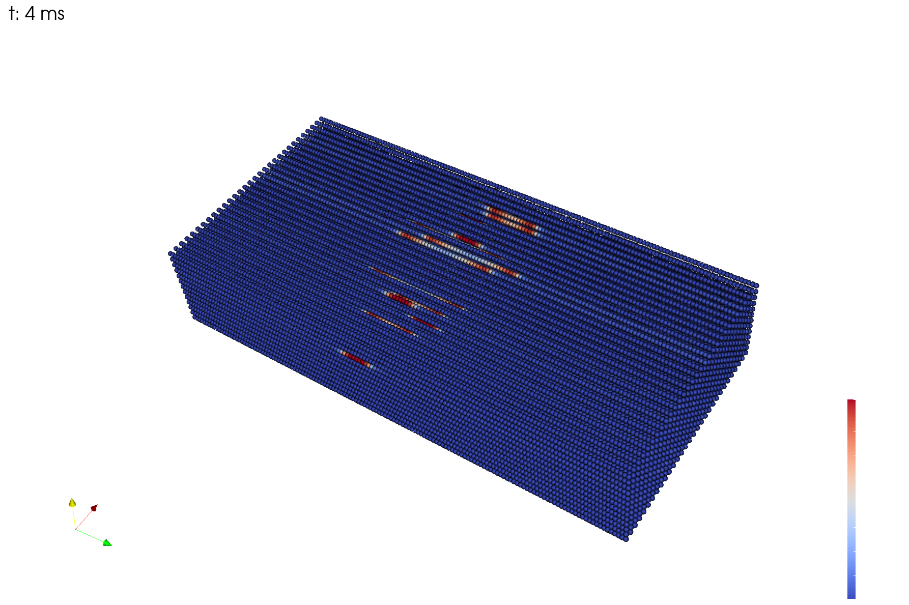
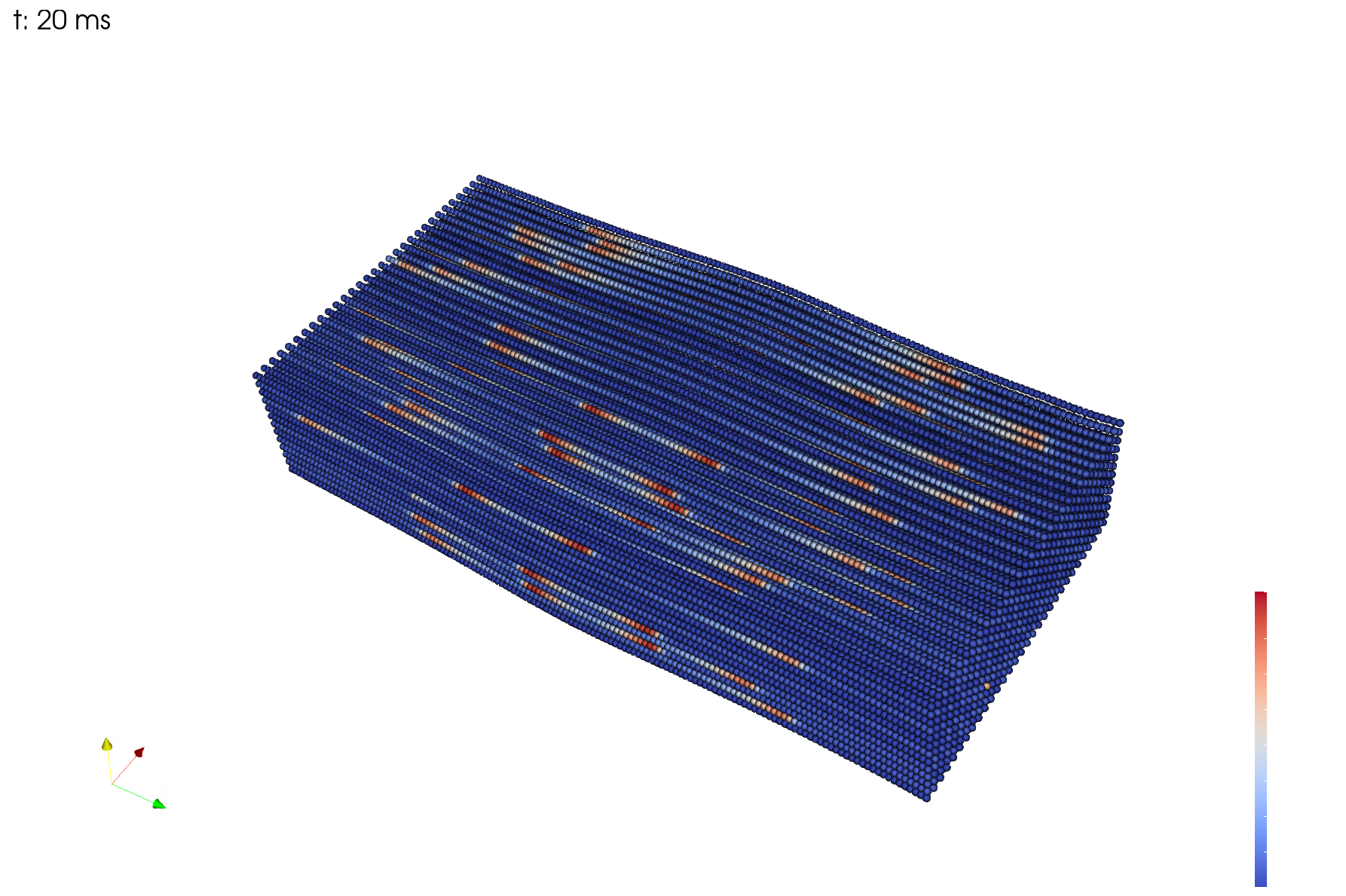
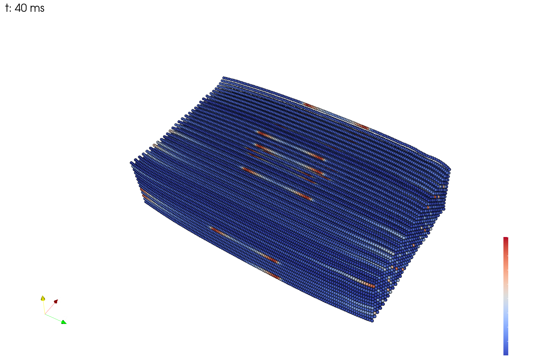
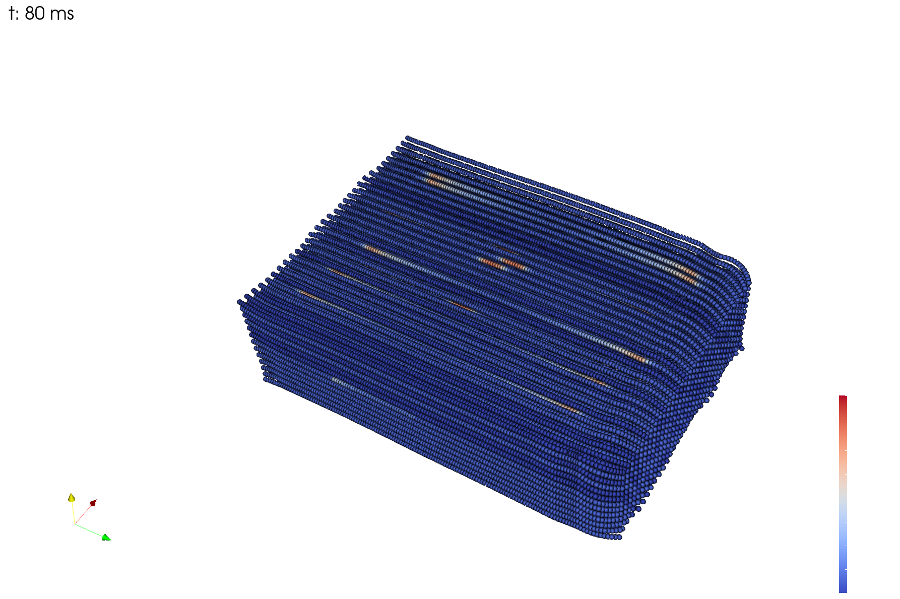
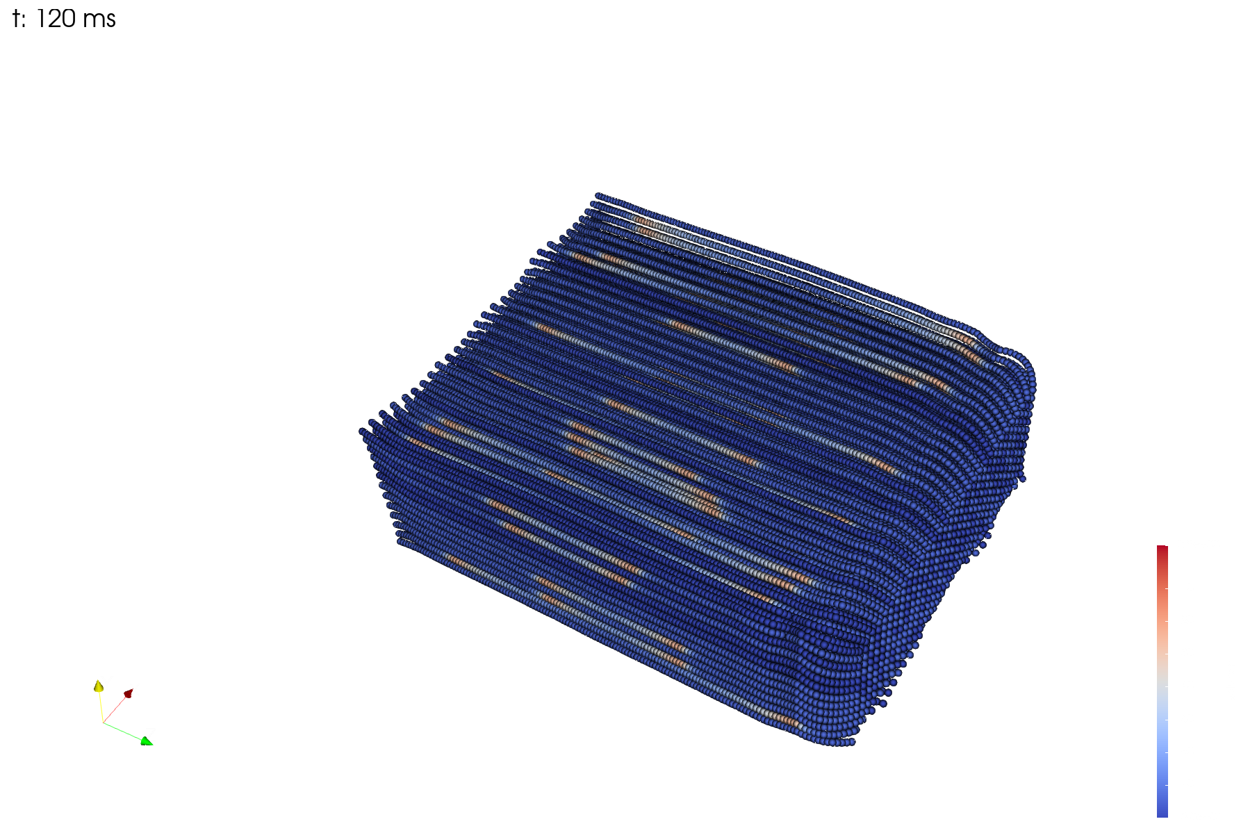
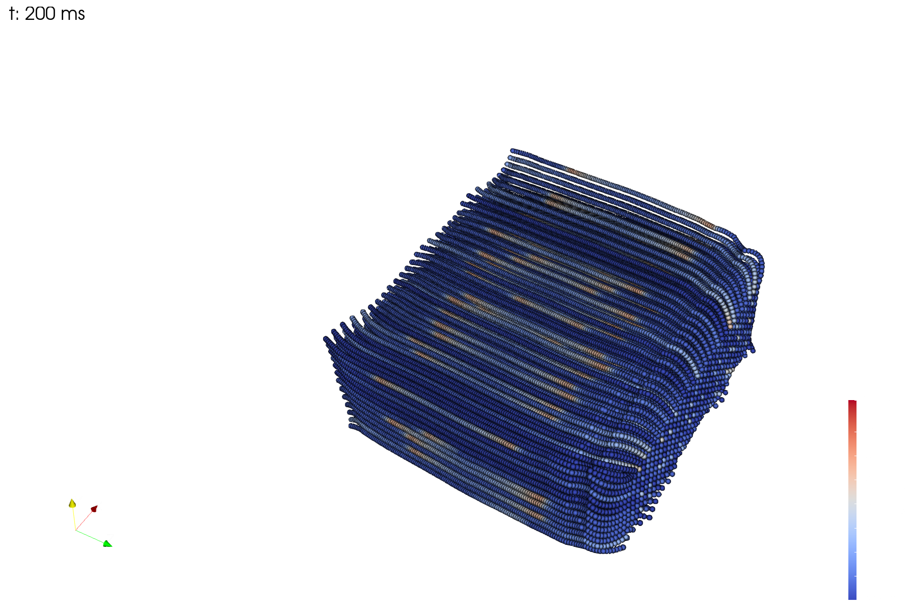
Fig. 95 evaluates the amount of contraction that the muscle undergoes in this scenario. The orange lines shows the average over all nodes of the 3D mesh, the light orange range corresponds to the 25%-75% quartile range of values. At 240ms, the average stretch is circa 90% which means that the muscle contracted by 10% in this time.
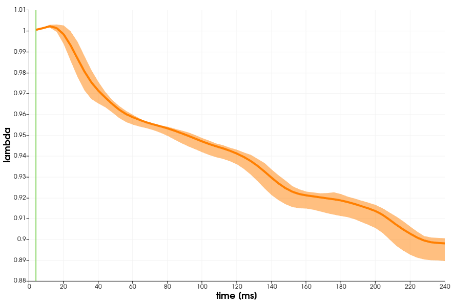
Fig. 95 Stretch over time of the muscle tissue.
More details about the scenario in OpenDiHu can be found here:
0/16 : This is opendihu 1.3, built Aug 29 2023, C++ 201402, GCC 9.4.0, current time: 2023/8/30 11:10:01, hostname: pcsgs05, n ranks: 16
0/16 : Open MPI v4.0.3, package: Debian OpenMPI, ident: 4.0.3, repo rev: v4.0.3, Mar 03, 2020
0/16 : File "../settings_cuboid_muscle.py" loaded.
0/16 : ---------------------------------------- begin python output ----------------------------------------
Loading variables from "heidlauf.py".
scenario_name: heidlauf,  n_subdomains: 2 2 4,  n_ranks: 16,  end_time: 4000.0
dt_0D:           1e-04, diffusion_solver_type:      cg
dt_1D:           1e-04, potential_flow_solver_type: gmres
dt_splitting:    1e-04, emg_solver_type:            cg, emg_initial_guess_nonzero: False
dt_3D:           1e+00, paraview_output: True
output_timestep: 1e+00  stimulation_frequency: 1.0 1/ms = 1000.0 Hz
fast_monodomain_solver_optimizations: True, use_analytic_jacobian: True, use_vc: True
fiber_file:              cuboid.bin
fat_mesh_file:           ../../../../input/13x13fibers.bin_fat.bin
cellml_file:             ../../../electrophysiology/input/new_slow_TK_2014_12_08.c
fiber_distribution_file: ../../../electrophysiology/input/MU_fibre_distribution_10MUs.txt
firing_times_file:       ../../../electrophysiology/input/MU_firing_times_heidlauf_10MU.txt
********************************************************************************
prefactor: sigma_eff/(Am*Cm) = 0.0132 = 3.828 / (500.0*0.58)
create cuboid.bin with size [2.9,1.2,6], n points [31,13,145]
diffusion solver type: cg
n fibers:              403 (31 x 13), sampled by stride 2 x 2
n points per fiber:    145, sampled by stride 4
16 ranks, partitioning: x2 x y2 x z4
31 x 13 = 403 fibers, per partition: 14 x 6 = 84
per fiber: 1D mesh    nodes global: 145, local: 36
  sampling 3D mesh with stride 2 x 2 x 4
  distribute_nodes_equally: True
quadratic 3D mesh    nodes global: 15 x 5 x 33 = 2475, local: 8 x 2 x 8 = 128
quadratic 3D mesh elements global: 7 x 2 x 16 = 224, local: 4 x 1 x 4 = 16
number of degrees of freedom:
                    1D fiber:        145  (per process: 36)
            0D-1D monodomain:       8120  (per process: 2016)
all fibers 0D-1D monodomain:    3272360  (per process: 169344)
                3D bidomain:       2475  (per process: 128)
                      total:    3274835  (per process: 169472)
Debugging output about fiber firing: Taking input from file "../../../electrophysiology/input/MU_firing_times_heidlauf_10MU.txt"
First stimulation times
    Time  MU fibers
    0.00   2 [60, 80, 81, 101, 104, 118, 127, 191, 228, 275] (only showing first 10, 19 total)
    2.00   3 [1, 12, 17, 40, 75, 76, 82, 94, 98, 108] (only showing first 10, 22 total)
    3.00   5 [7, 10, 19, 21, 24, 32, 35, 43, 62, 68] (only showing first 10, 42 total)
    7.01   4 [14, 16, 27, 39, 52, 106, 111, 116, 125, 146] (only showing first 10, 35 total)
    8.01   7 [0, 2, 9, 15, 18, 28, 33, 36, 45, 55] (only showing first 10, 53 total)
    9.01   1 [29, 49, 58, 102, 131, 134, 153, 182, 184, 232] (only showing first 10, 14 total)
  16.02   6 [26, 31, 44, 51, 53, 56, 57, 65, 67, 83] (only showing first 10, 46 total)
  35.04   8 [3, 13, 23, 25, 30, 38, 41, 54, 71, 78] (only showing first 10, 69 total)
  never stimulated: MU   0, fibers [37, 46, 47, 48, 69, 74, 89, 93, 138, 213] (only showing first 10, 23 total)
stimulated MUs: 8, not stimulated MUs: 1
How to reproduce
Build the example
cd $OPENDIHU_HOME/opendihu/examples/validation/cuboid_muscle/
mkorn && sr
Run the simulation
cd $OPENDIHU_HOME/opendihu/examples/validation/cuboid_muscle/build_release
mpirun -n 16 ./cuboid_muscle ../settings_cuboid_muscle.py heidlauf.py