In the following all (or at least the most important) examples are listed. The order corresponds to the directory structure under opendihu/examples.
The most examples can be run with any number of processes.
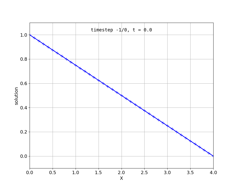
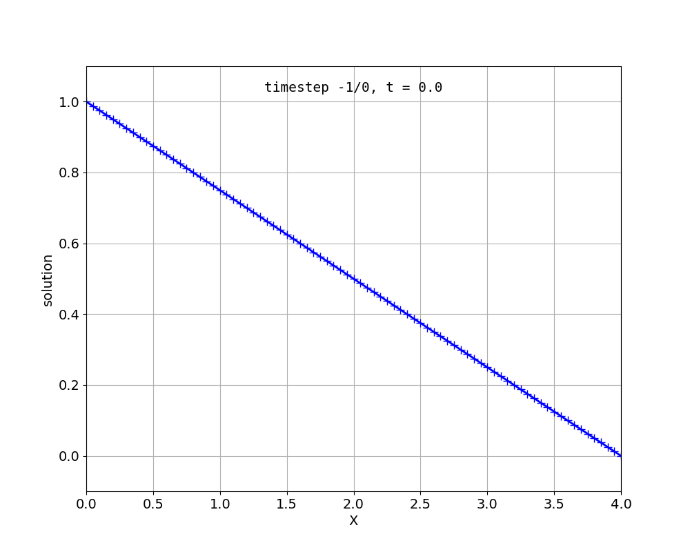
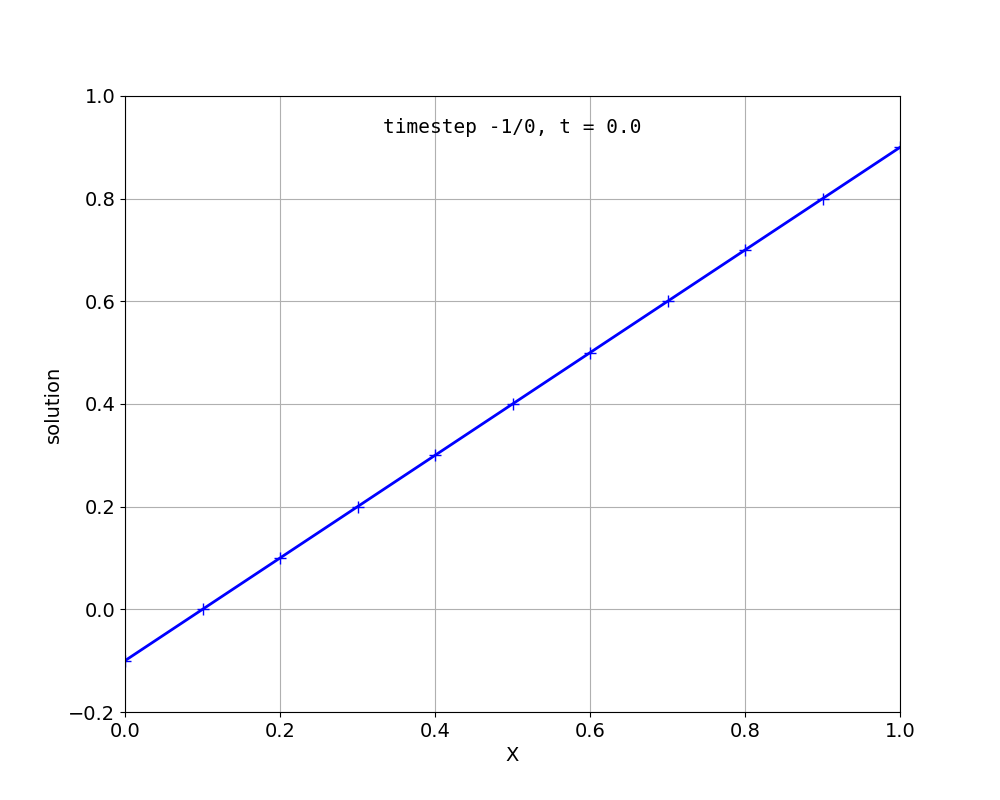
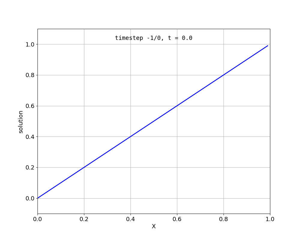
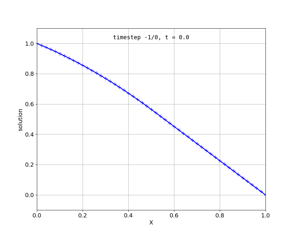
This solves the laplace equation on a line, with linear and quadratic Lagrange ansatz functions or cubic Hermite ansatz functions. Neumann and Dirichlet-type boundary conditions are used.
Output files will be written in the out subdirectory. The *.py files can be visualized by running plot. The *.vtr file can be viewed with paraview. System matrices, solution and rhs vectors are dumped in matlab format.
This solves the 2d laplace equation, with linear and quadratic Lagrange ansatz functions or cubic Hermite ansatz functions. laplace_hermite demonstrates how to use unstructured grids.
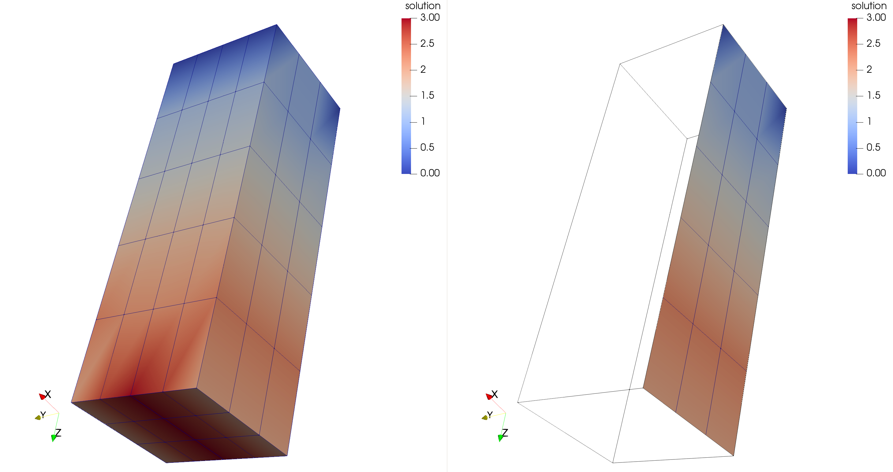
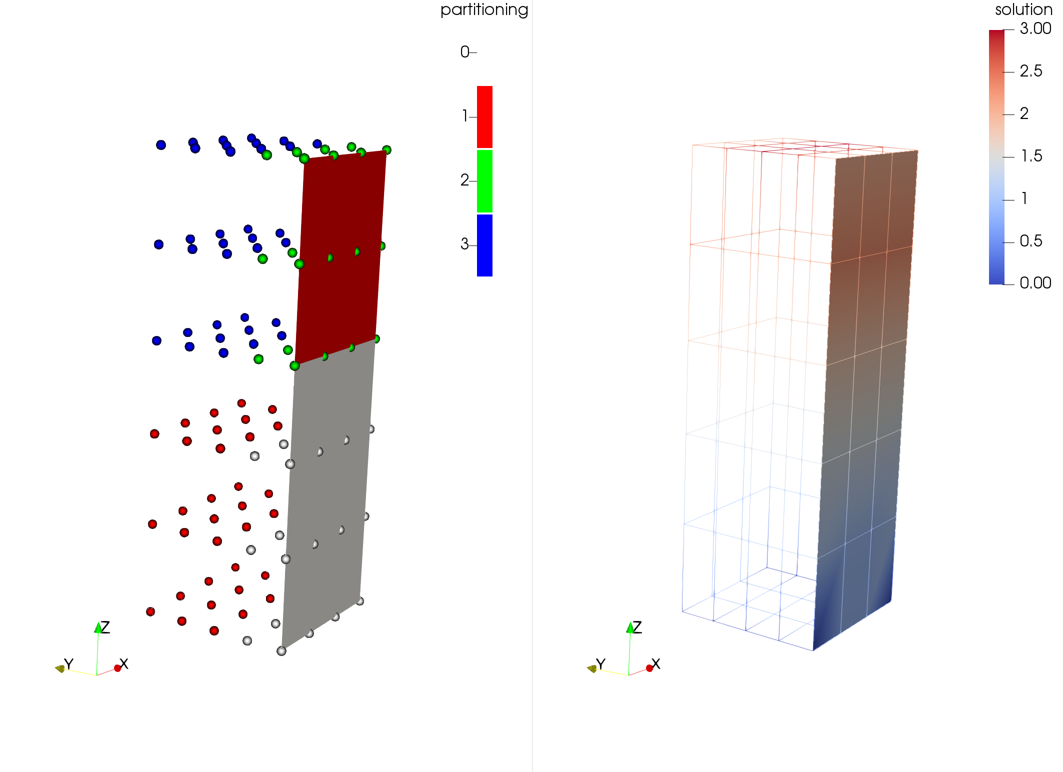
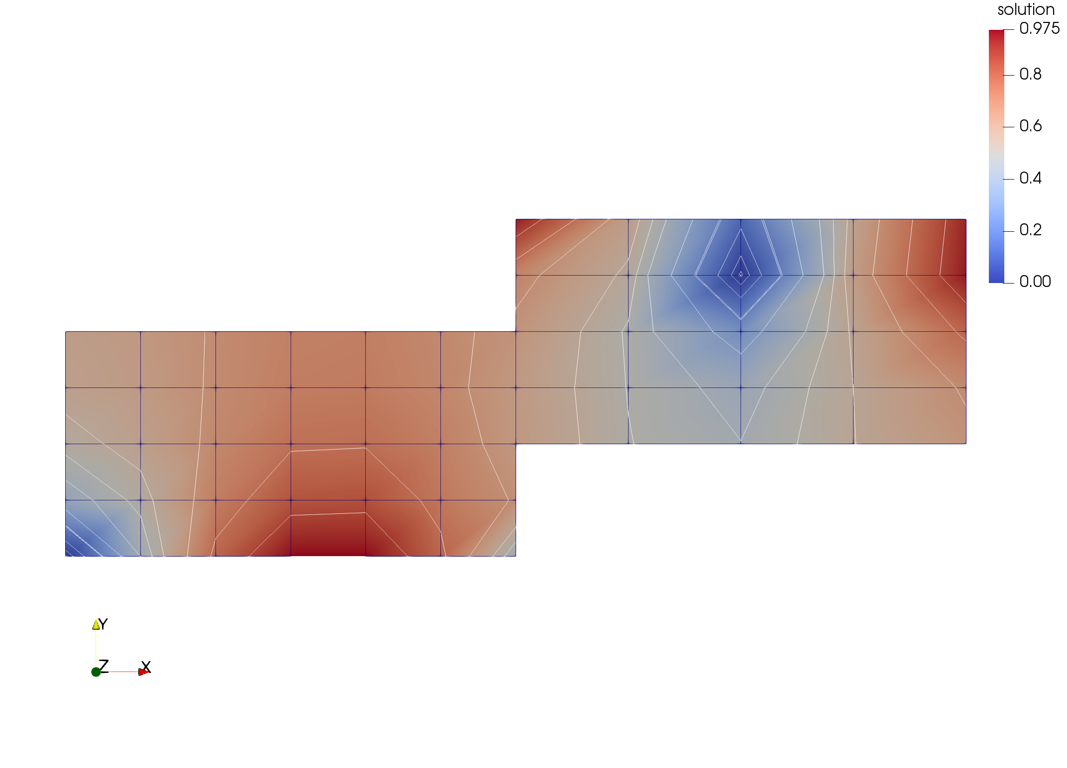
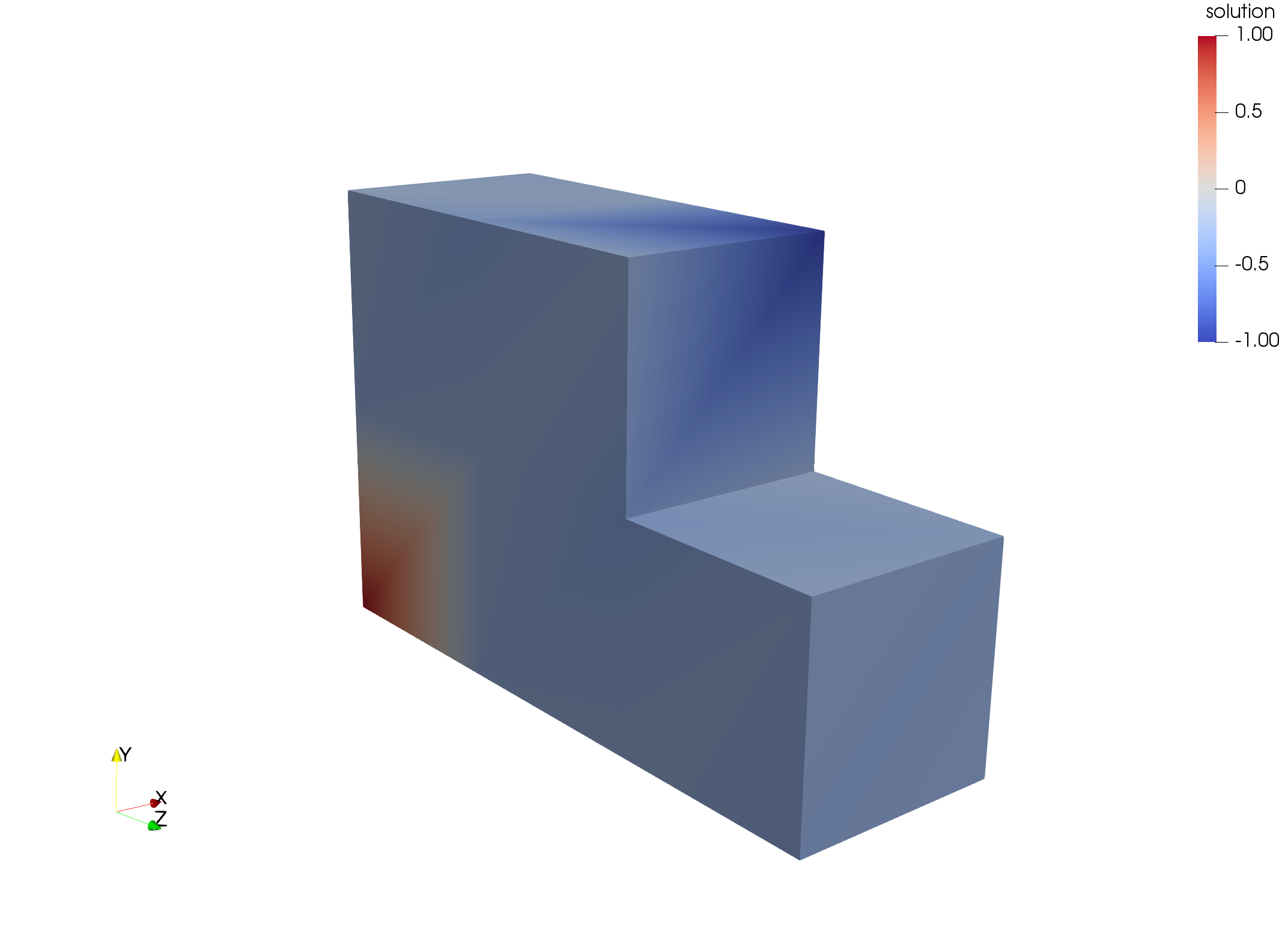
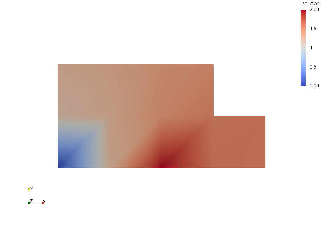
Solve the 3D Laplace problem and demonstrate how to use :doc:/settings/output_surface to extract a surface. This is needed if the full 3D data would be too large to output, but a 2D surface is okay.
Fig. 12 Scenario (1). Left: the full mesh, right: only surface as written by the OutputSurface writer.
Fig. 13 Scenario (2). This shows that it also works with parallel execution (4 processes). Note how the surface is only written by two processes, whereas the volume is written by all 4 processes.
Output files will be written in the out subdirectory. The *.py files can be visualized by running plot. The written rhs vector in poisson_rhs_000.txt is the weak form of the rhs!
Output files will be written in the out subdirectory. The *.py files can be visualized by running plot. The written rhs vector in poisson_rhs_000.txt is the weak form of the rhs!
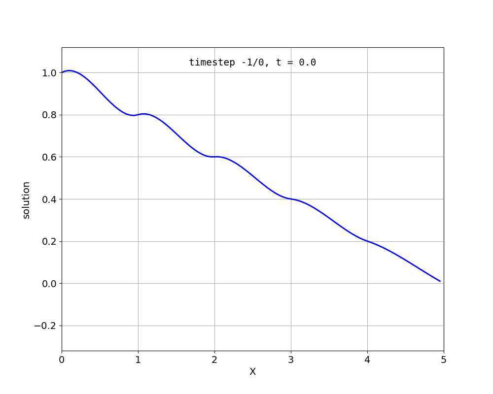
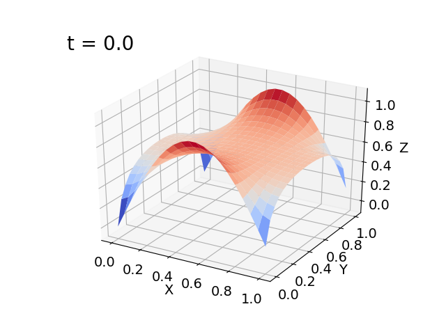
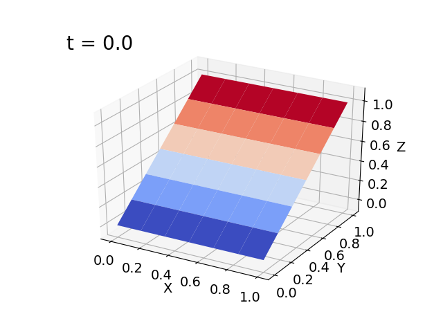
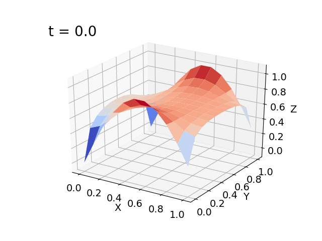
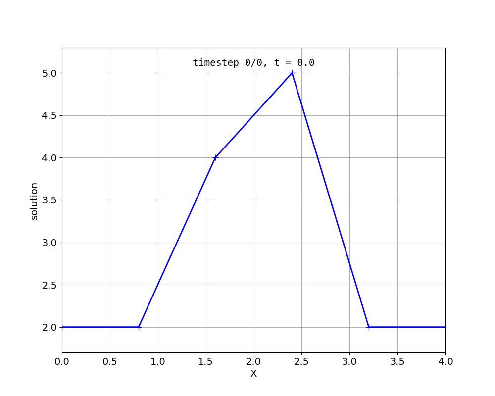
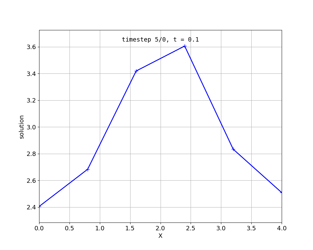
again with Dirichlet or Neumann-type boundary conditions and different initial values. There are again versions for different dimensionalities, diffusion1d, diffusion2d and diffusion3d`.
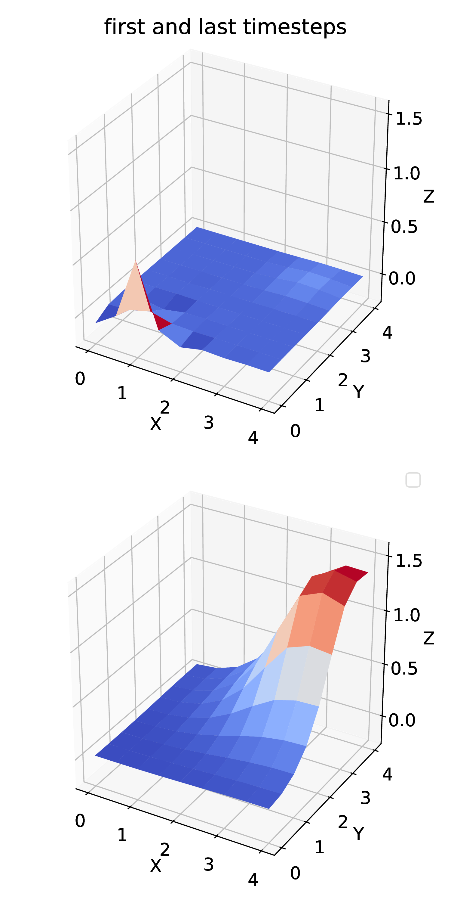
This solves the diffusion equation with source term
\[u_t - cΔu = f(t)\]
with a source function \(f(x,t)\). This function defined in the python settings as callback function. This example demonstrates how to use the PrescribedValues class.
(Actually this is not a reaction diffusion equation, because \(f\) does not depend on \(u\).)
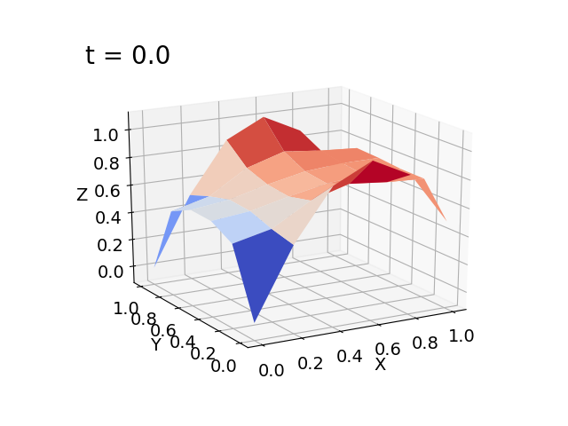
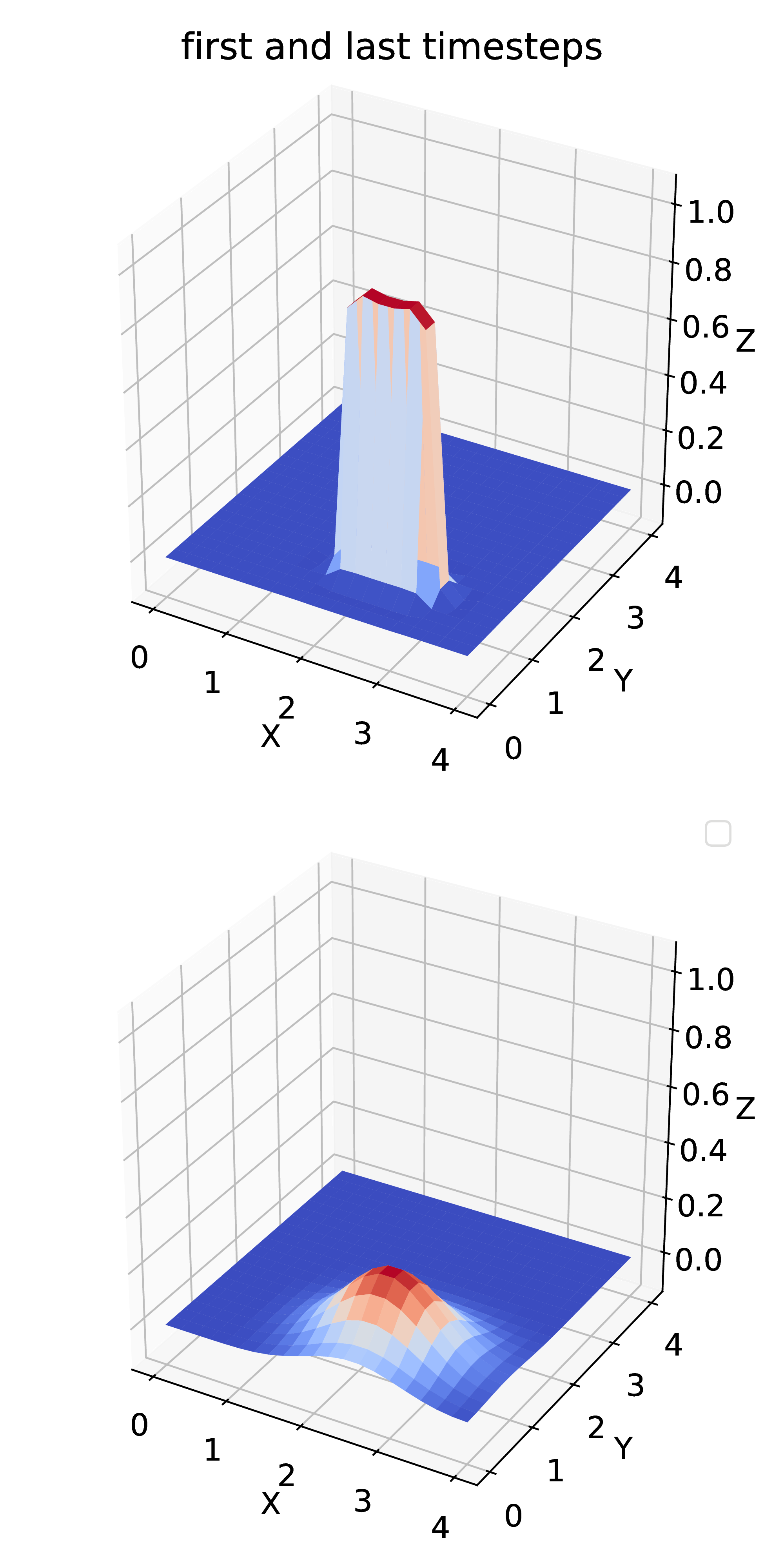
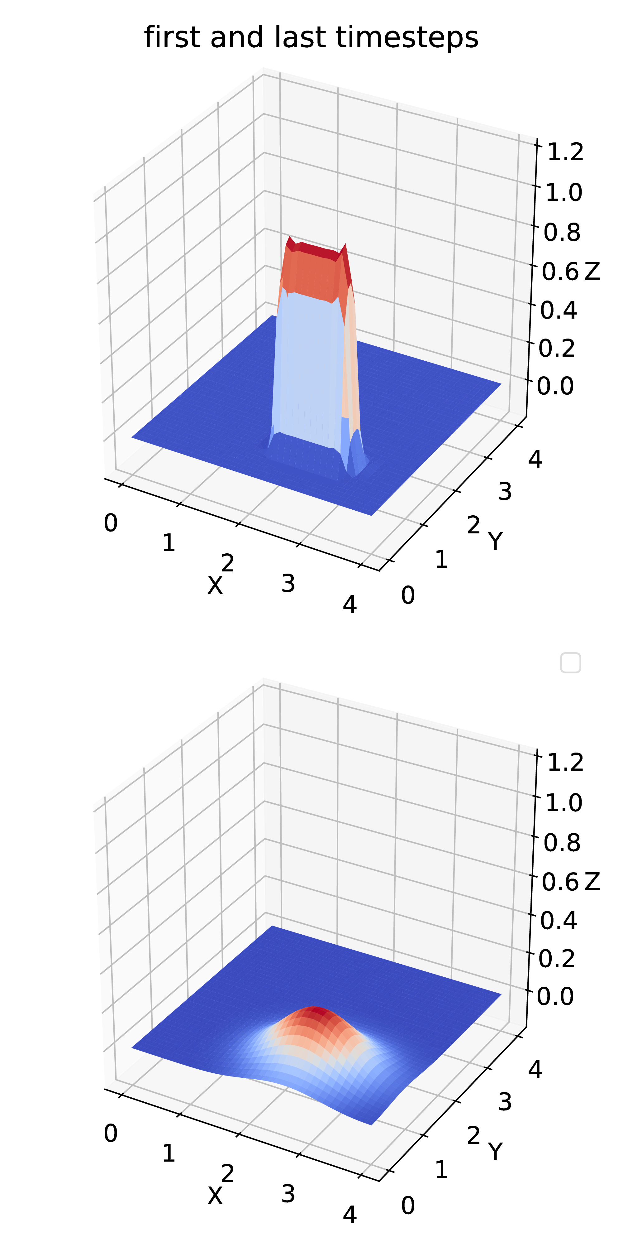
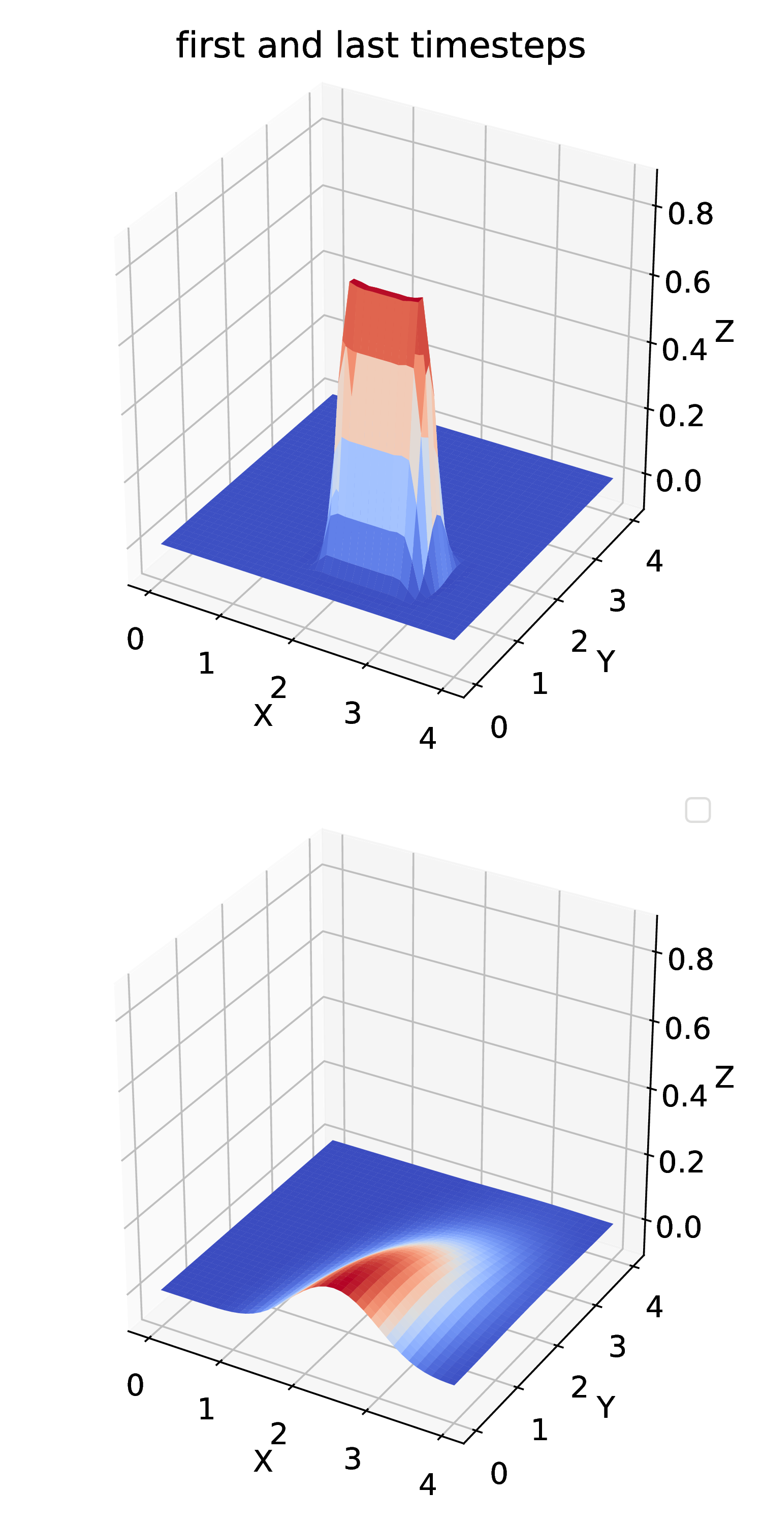
Fig. 24 Scenarios (1) and (2) produce the same results. Here, it makes sense to run plot in the out folder, to see the animation. The small peak at \((0.55,0.25)\) diffuses away, the callback function places a constant source at around \((2.8,2.8)\) which leads to the new maximum in the last timestep.
1D diffusion problem using the parallel-in-time algorithm “Multigrid reduction in time” (MGRIT) for the solution. This was done in the master thesis of Marius Nitzsche.
Functionality to create fiber geometry for the Biceps Brachii muscle from a surface mesh of the muscle. This is very sophisticated and can be run in parallel.
This is the parallel algorithm that creates the fiber meshes. Input is an STL mesh of the surface of the muscle volume. Output is a *.bin file of the mesh.
Use the following commands to compile the program:
Which input file to choose. If set to splines, the input file is ../../../electrophysiology/input/biceps.surface.pickle, otherwise it is ../../../electrophysiology/input/biceps_splines.stl.
refinement
(Integer), how to refine the mesh prior to solving the Laplace problem. 1 means no refinement, 2 means half the mesh width, 3 third mesh width etc.
improve_mesh
Either true or false. If the 2D meshes on the slices should be smoothed, i.e. improved. If true, it takes longer but gives better results.
use_gradient_field
Either true or false. If the tracing implementation using explicit gradient fields should be used.
use_neumann_bc
Either true or false. If Neumann boundary conditions should be used for the Laplacian potential flow problem. If not, Dirichlet boundary conditions are used.
with shear modulus \(\mu\) and bulk modulus \(K\).
It shows how the normal FiniteElementMethod class can be used for this problem.
For scenarios (3), (4) and (5), an active stress term is additionally considered, such that the 2nd Piola-Kirchhoff stress tensor is given as \(S = S_\text{passive} + S_\text{active}\).
cd$OPENDIHU_HOME/examples/solid_mechanics/linear_elasticity/box
mkorn&&sr# buildcdbuild_release
./linear_elasticity_2d../settings_linear_elasticity_2d.py# (1)
./linear_elasticity_3d../settings_linear_elasticity_3d.py# (2)cd$OPENDIHU_HOME/examples/solid_mechanics/linear_elasticity/with_3d_activation
mkorn&&sr# buildcdbuild_release
./lin_elasticity_with_3d_activation_linear../settings.py# (3)
./lin_elasticity_with_3d_activation_quadratic../settings.py# (4) does not convergecd$OPENDIHU_HOME/examples/solid_mechanics/linear_elasticity/with_fiber_activation
mkorn&&sr# buildcdbuild_release
./lin_elasticity_with_fibers../settings_fibers.py# (5)
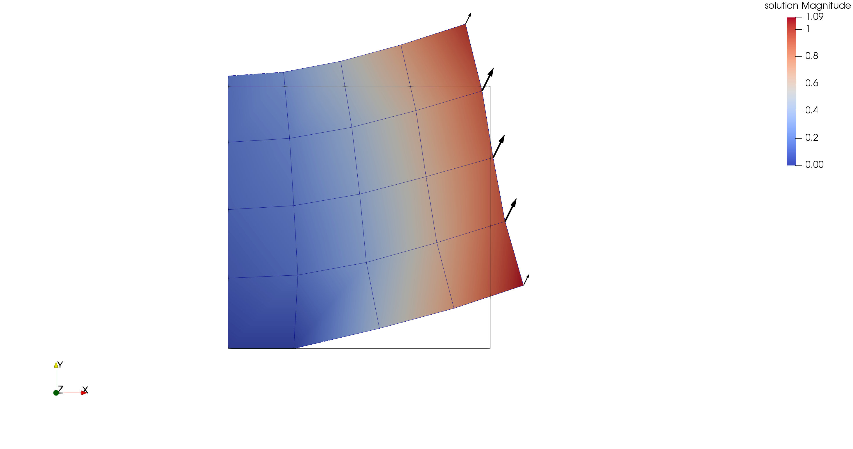
Fig. 25 Scenario (1): Neumann boundary conditions as black arrows (traction). This has been visualized using Arrow Glyphs and Warp filters in ParaView.
Fig. 26 Scenario (2): Neumann boundary conditions as black arrows (traction). This has been visualized using Arrow Glyphs and Warp filters in ParaView.
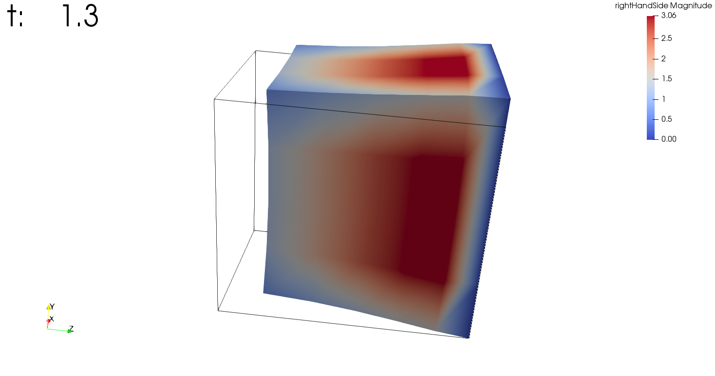
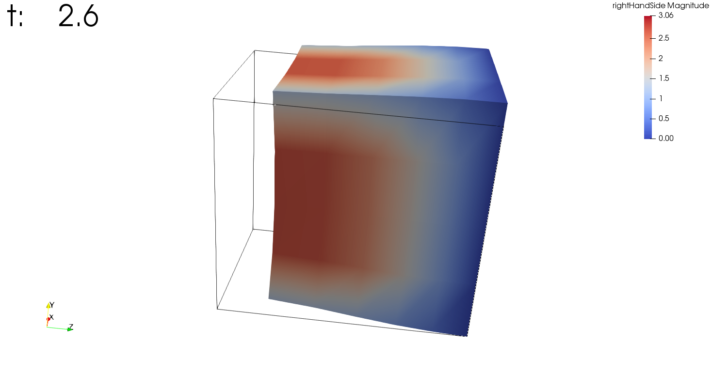
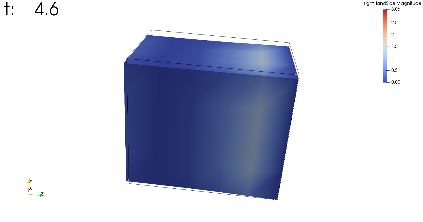
Scenario (3): This is a dynamic problem. An active stress value is prescribed over time in the 3D mesh and used in the elasticity computation. This simulates a periodically contracting muscle.
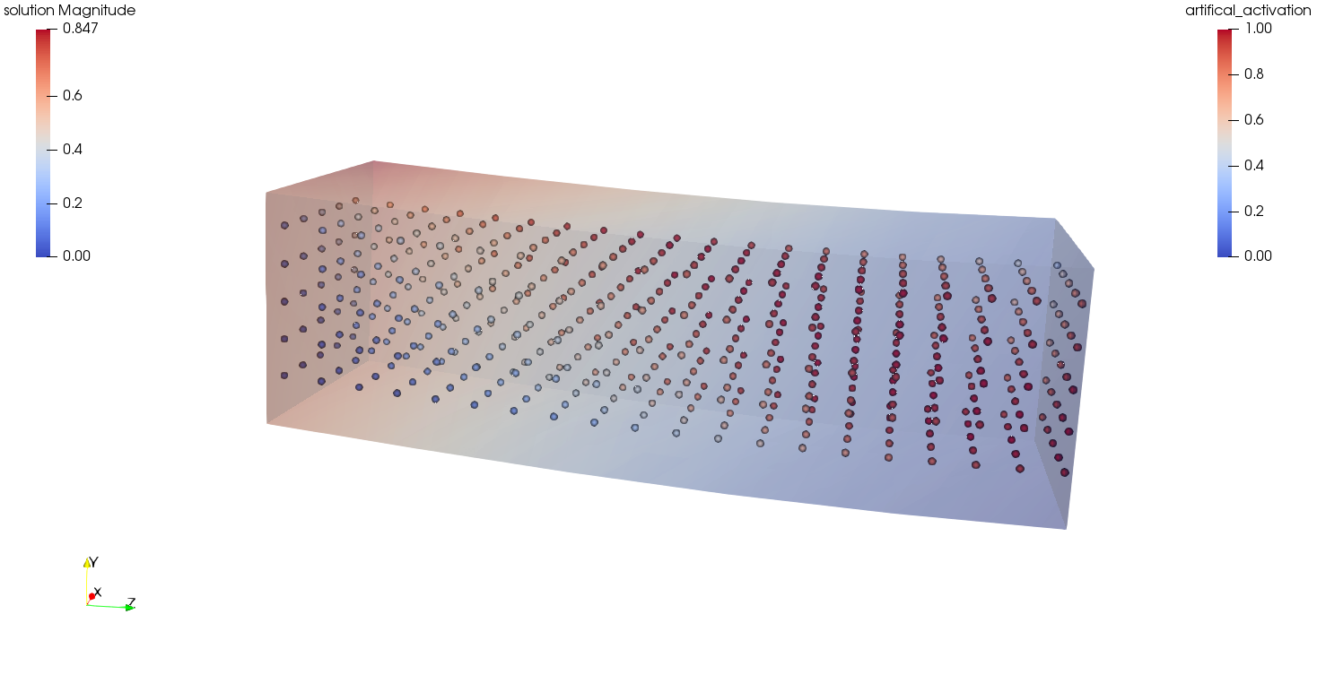
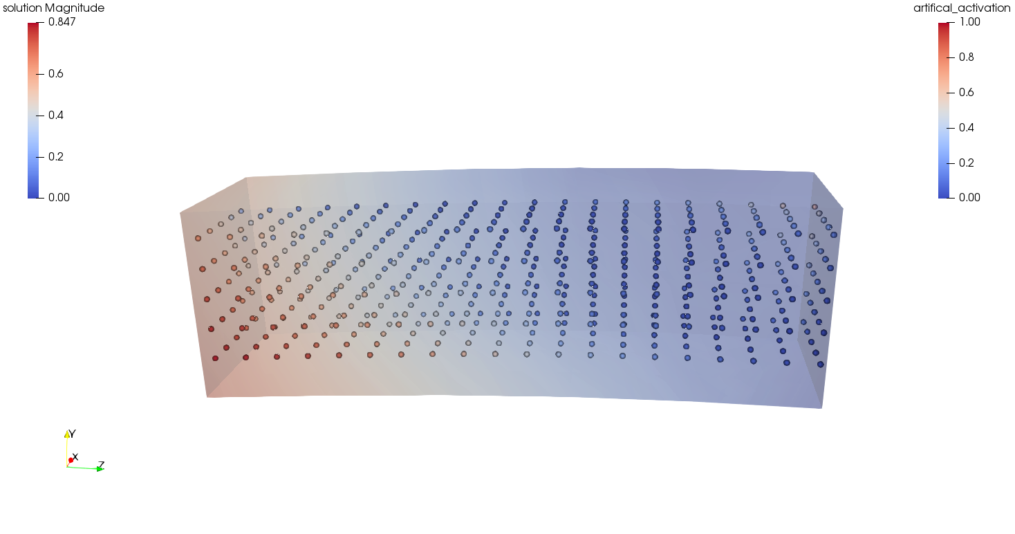
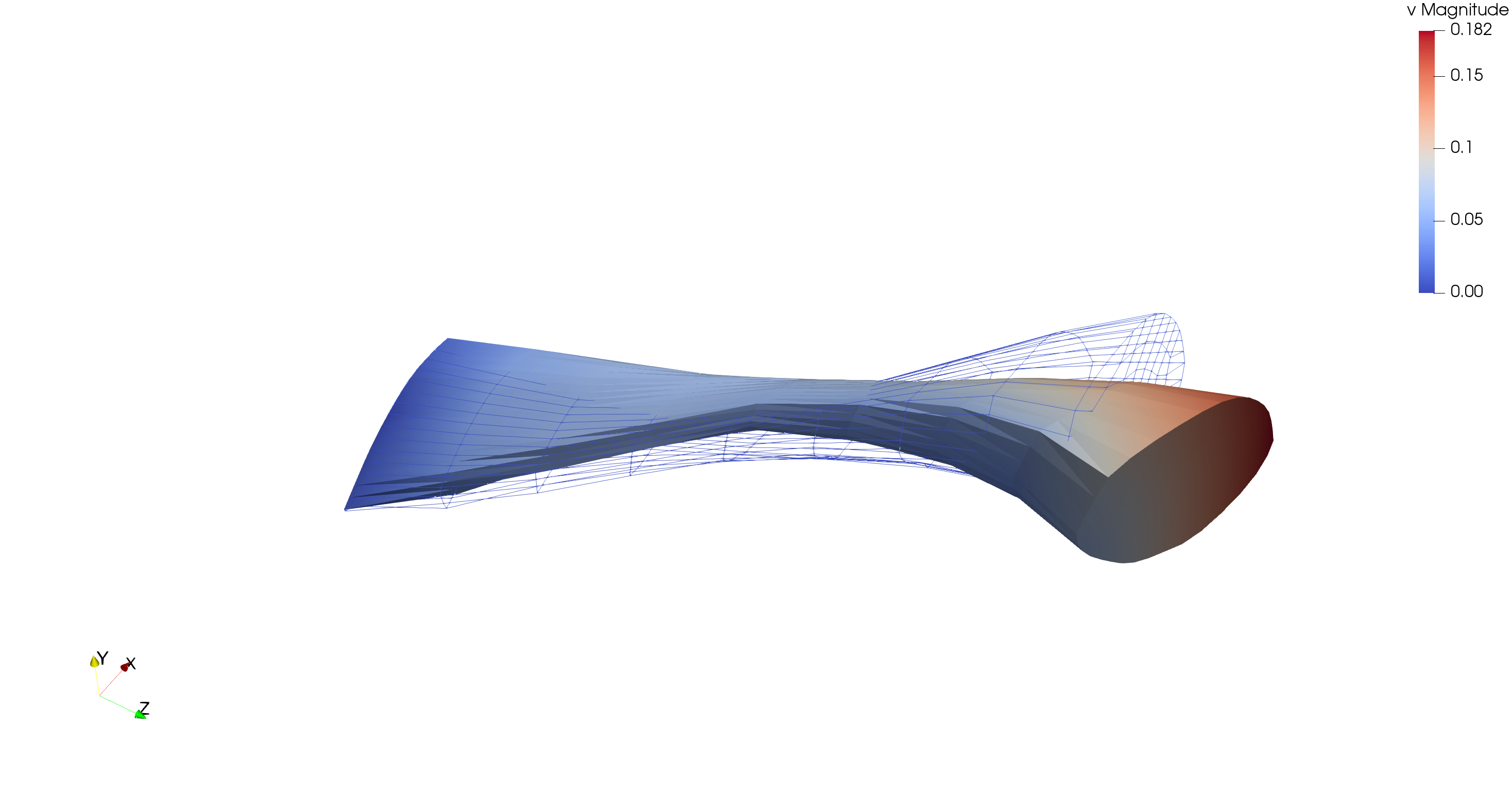
Scenario (5): An active stress value is prescribed over time at multiple 1D fibers (shown as spheres). This value gets mapped to the 3D mesh and used in the elasticity computation. This can also be seen as muscle tissue, which is bending up and down periodically.
Solves a static 3D nonlinear, incompressible solid mechanics problem with Mooney-Rivlin material. The strain energy function is formulated using the reduced invariants as follows.
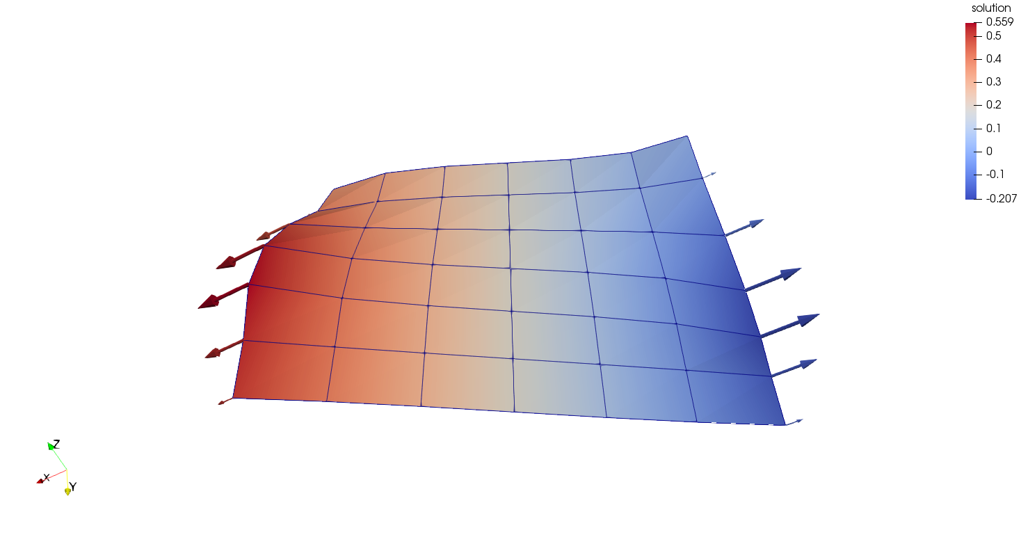
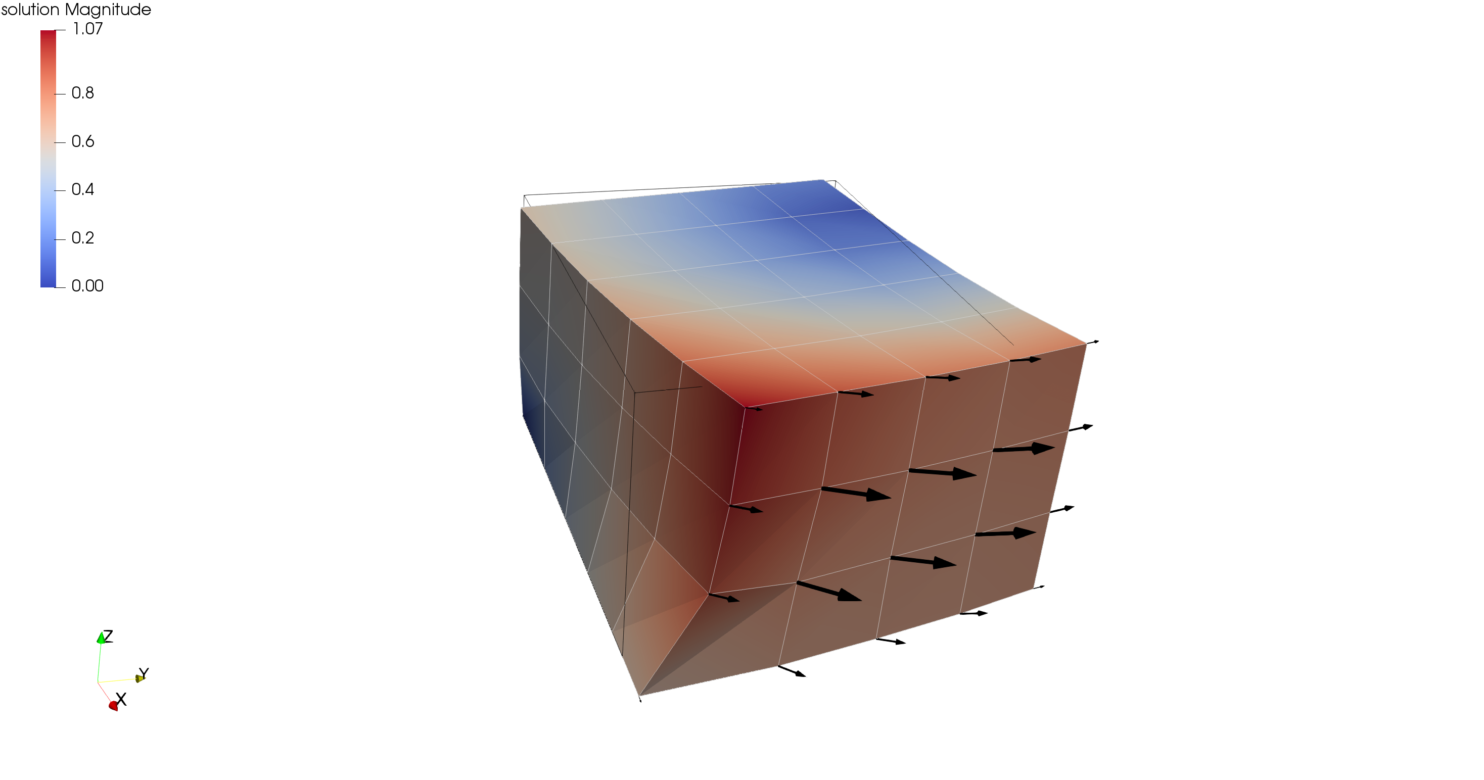
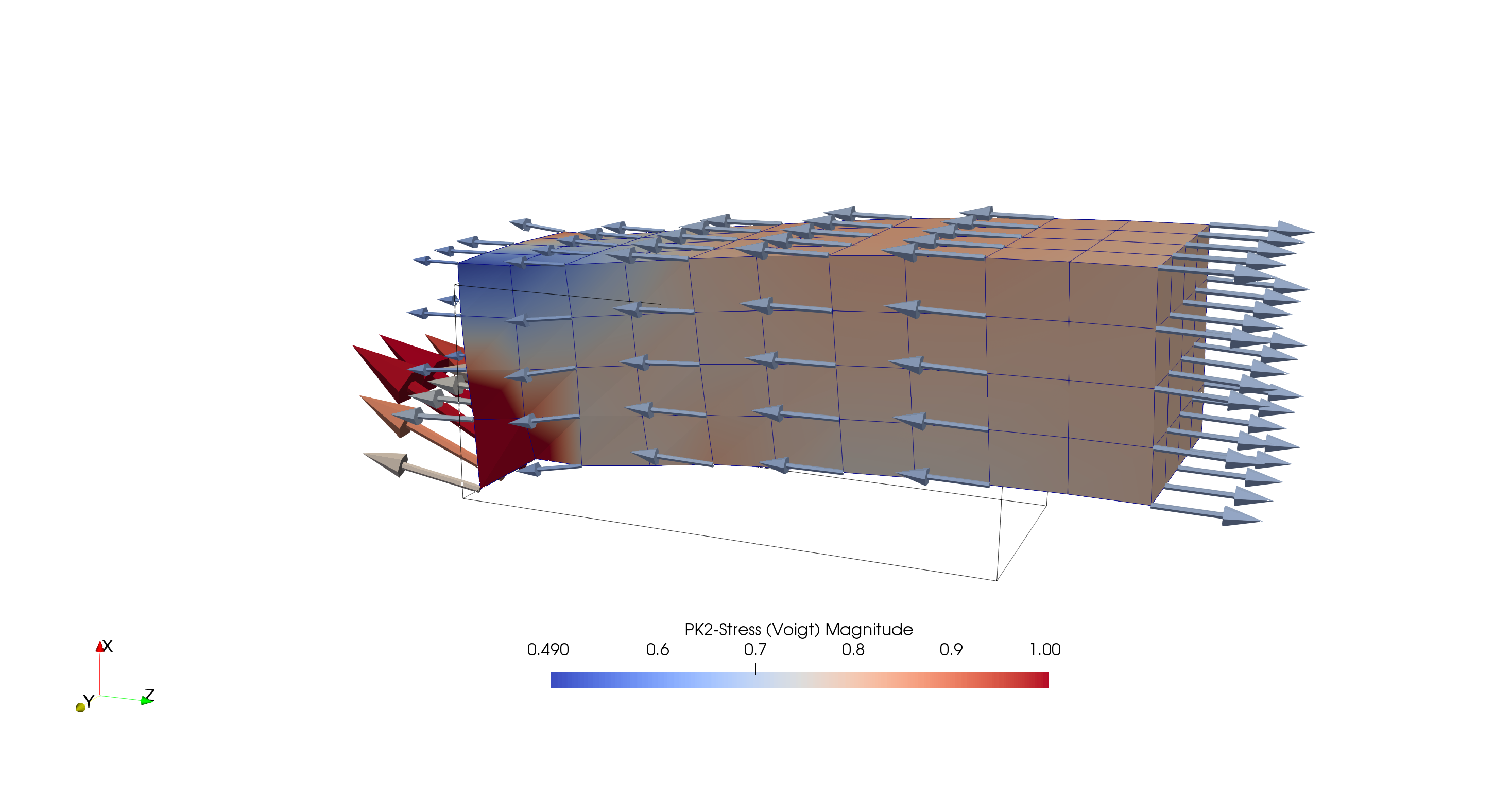
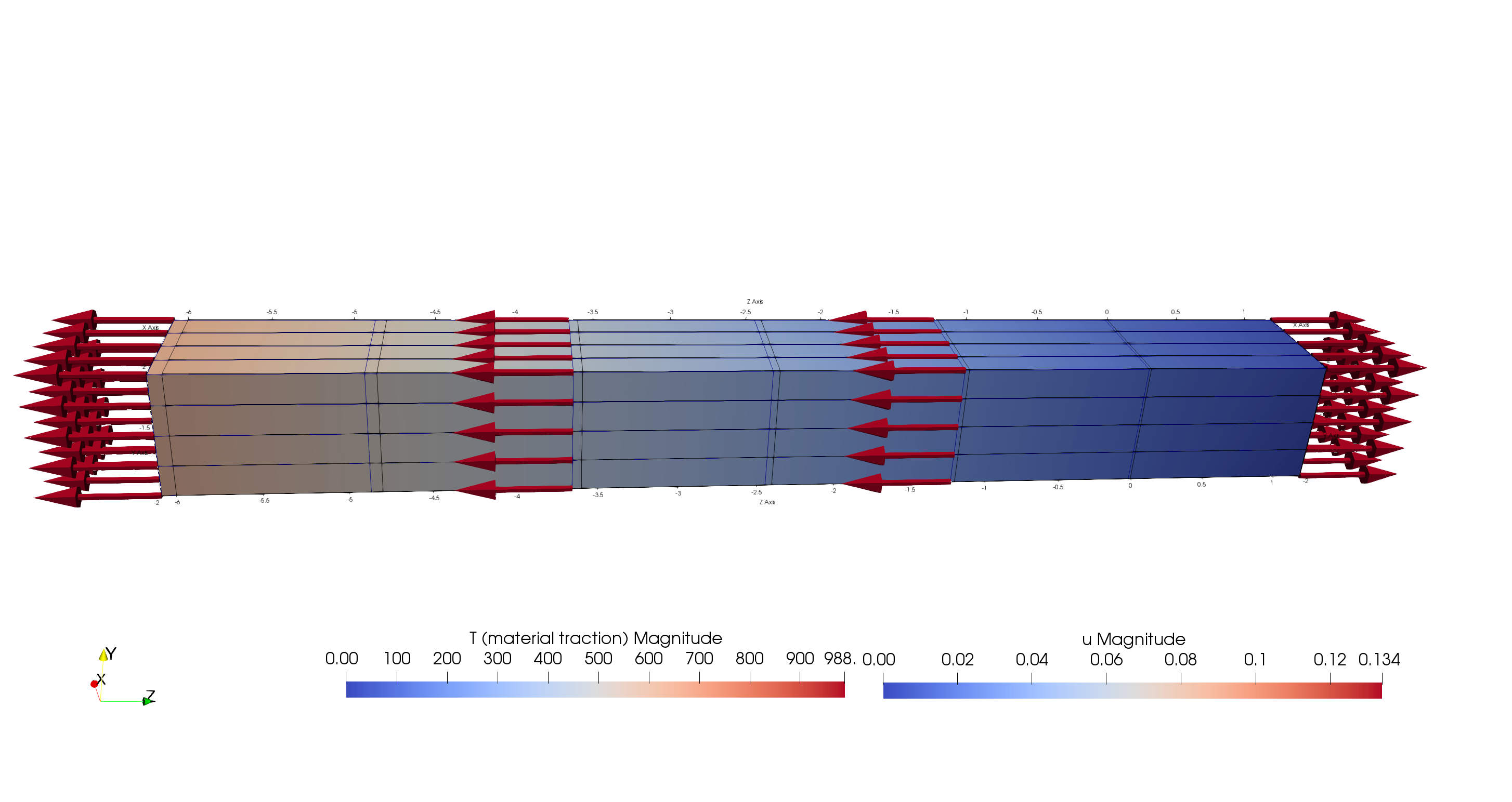
Fig. 27 Scenario (1): A deformed box, material parameters \(c_1=0, c_2=1\). The box is fixed at the left plane. The arrows visualize the traction.
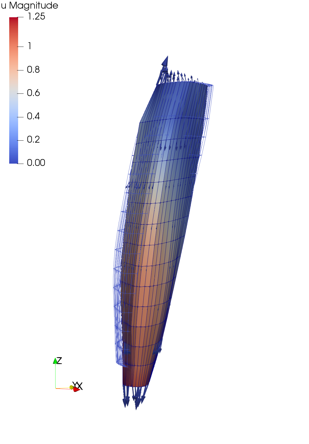
Fig. 28 Scenario (2): A deformed muscle geometry. Material parameters \(c_1 = 3.176e-10, c_2 = 1.813\) [N/cm^2]. The muscle is fixed at the top end, a force acts at the bottom end.
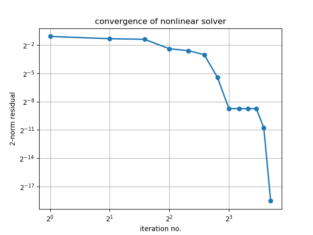
Fig. 29 The residual norm of the nonlinear solver over time steps. The Jacobian matrix is formed analytically every 5th iteration, in total three times (before iterations 1, 6, 11). It can be seen that the residual norm drops after every new Jacobian and then only increases a little more.
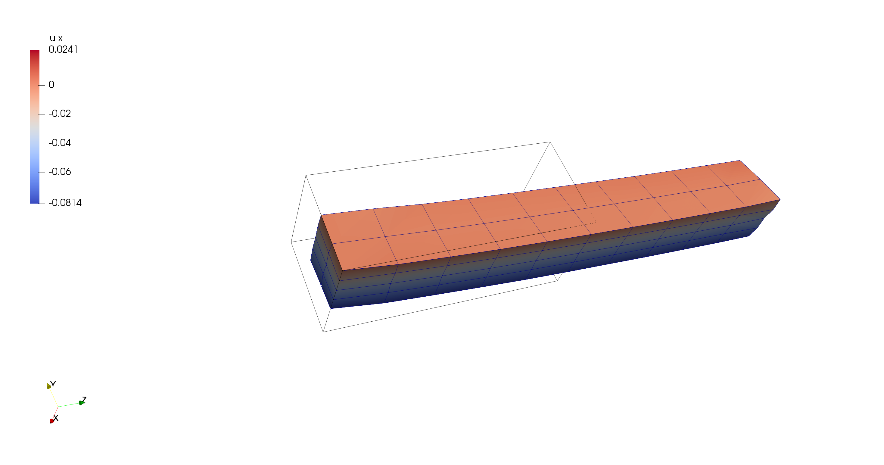
Fig. 30 Scenario (1): A deformed box. The box is fixed at the left plane, it contains diagonal internal fibers that are oriented by 40 degrees away from the center line. Material parameters are \(c_1=2, c_2=3, b_1=4, d_1=5\). The rod is only pulled towards the right, not to the bottom. The displacements are enlarged by the factor 10. It can be seen that by the anistropic material, it behaves asymmetrically.
Fig. 31 Scenario (2): A deformed muscle geometry, material parameters \(c_1 = 3.176e-10, c_2 = 1.813, b = 1.075e-2, d = 9.1733\). The muscle is fixed at the left end and pulled upwards by a force of 0.1 N.
Scenario (2): A piece of gelatine the gets moved to the right. This is realized with Dirichlet boundary conditions that can be updated over time by a python callback function.
With this scenario, we can demonstrate the effect of the option extrapolateInitialGuess. It controls whether the initial guess for the vector of unknowns in the dynamic solid mechanics problem is extrapolated from the two previous time steps.
We consider a simulation until \(t=10\) (set end_time=10 in settings_gelatine1.py).
At timestep 19 (\(t=9.5\)), we observe the following behaviour:
Table 1 Effect of extrapolating the initial guess
"extrapolateInitialGuess":
False
True
Initial residuum at \(t=9.5\)
8.07862
1.80136
Number of Newton iterations *)
5
3
Wall user time of the entire simulation
52 s
40 s
*): Number of Newton iterations of the
dynamic problem at \(t=9.5\), until the absolute error is below 1e-5.
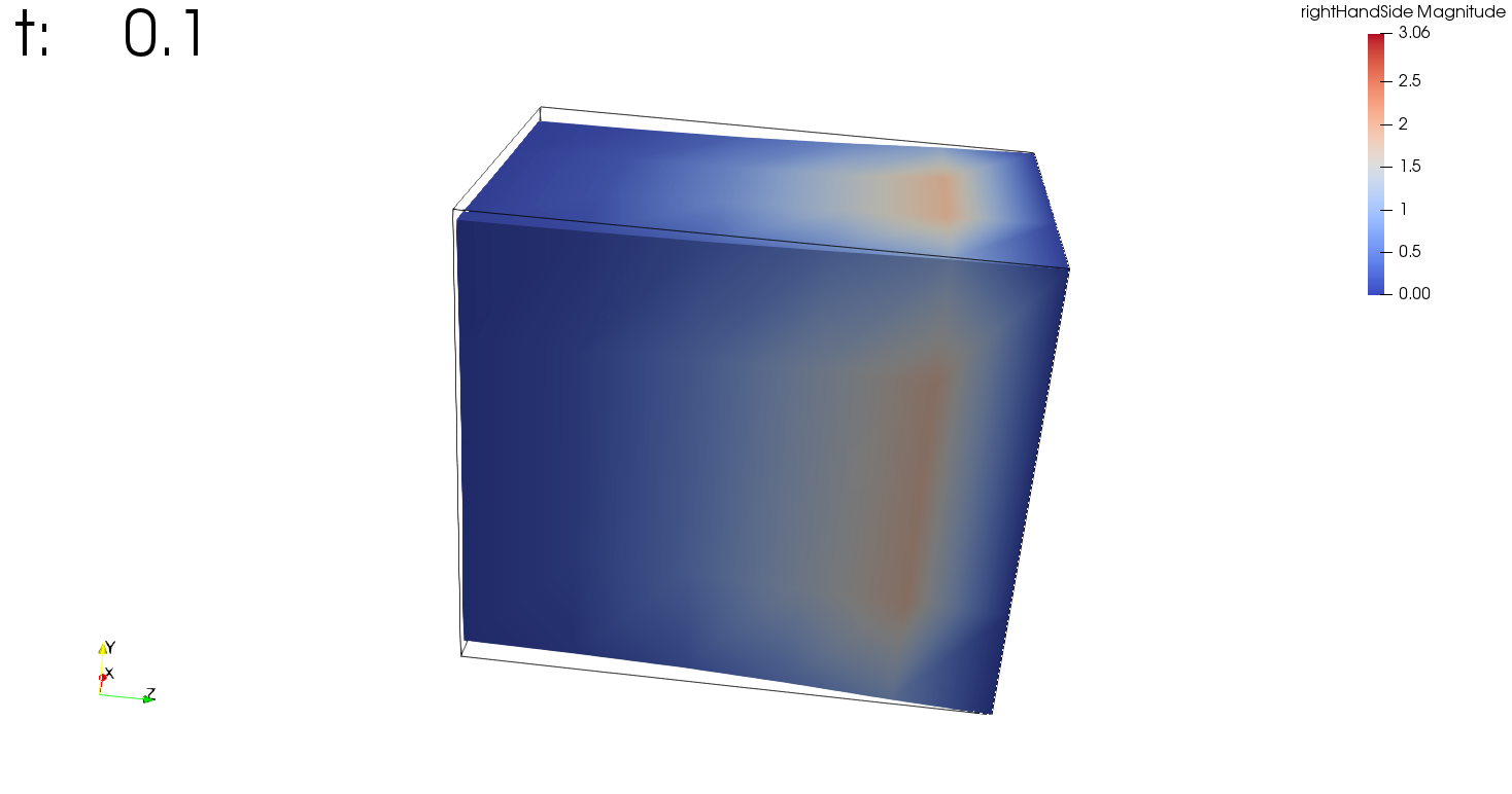
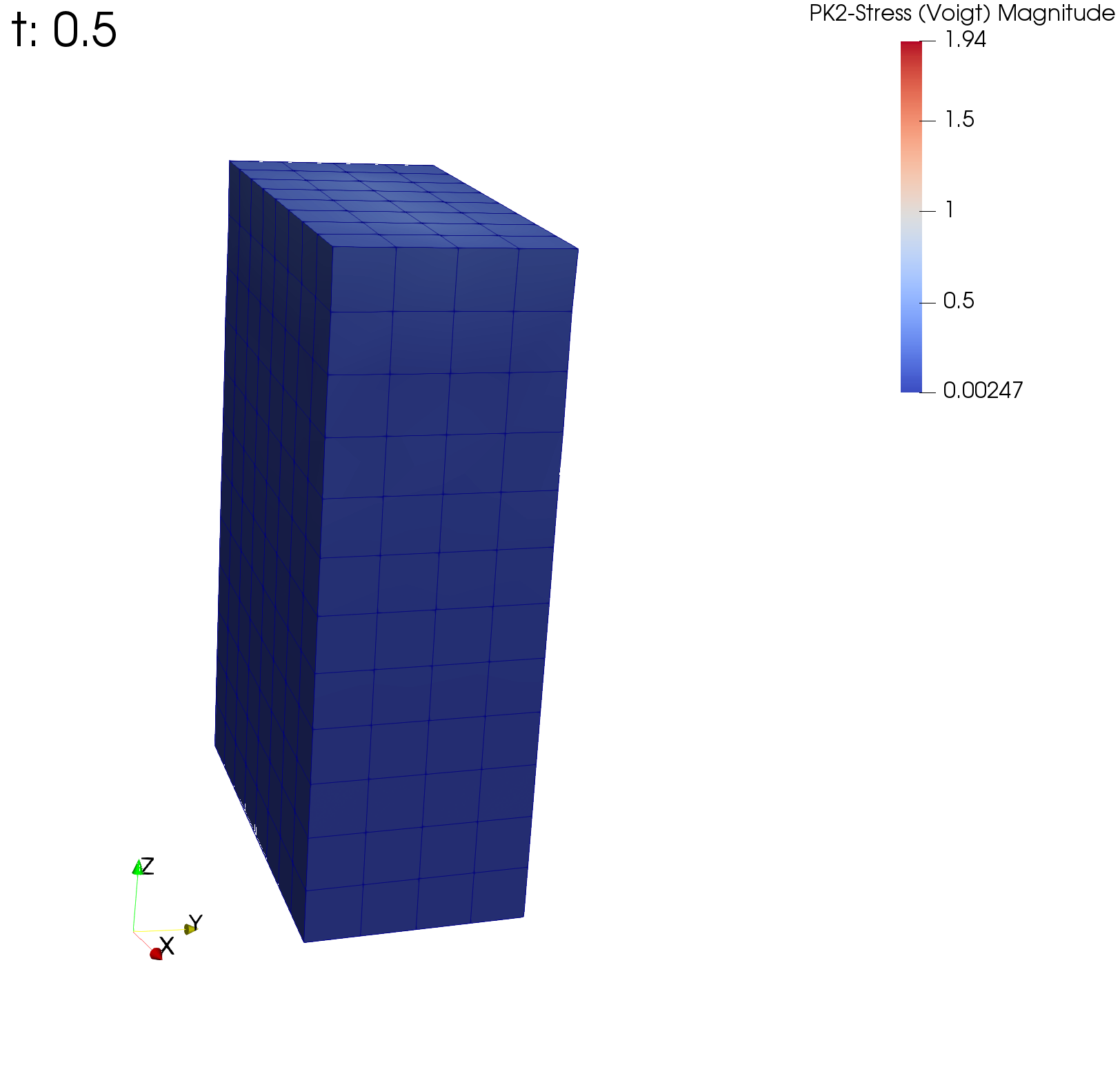
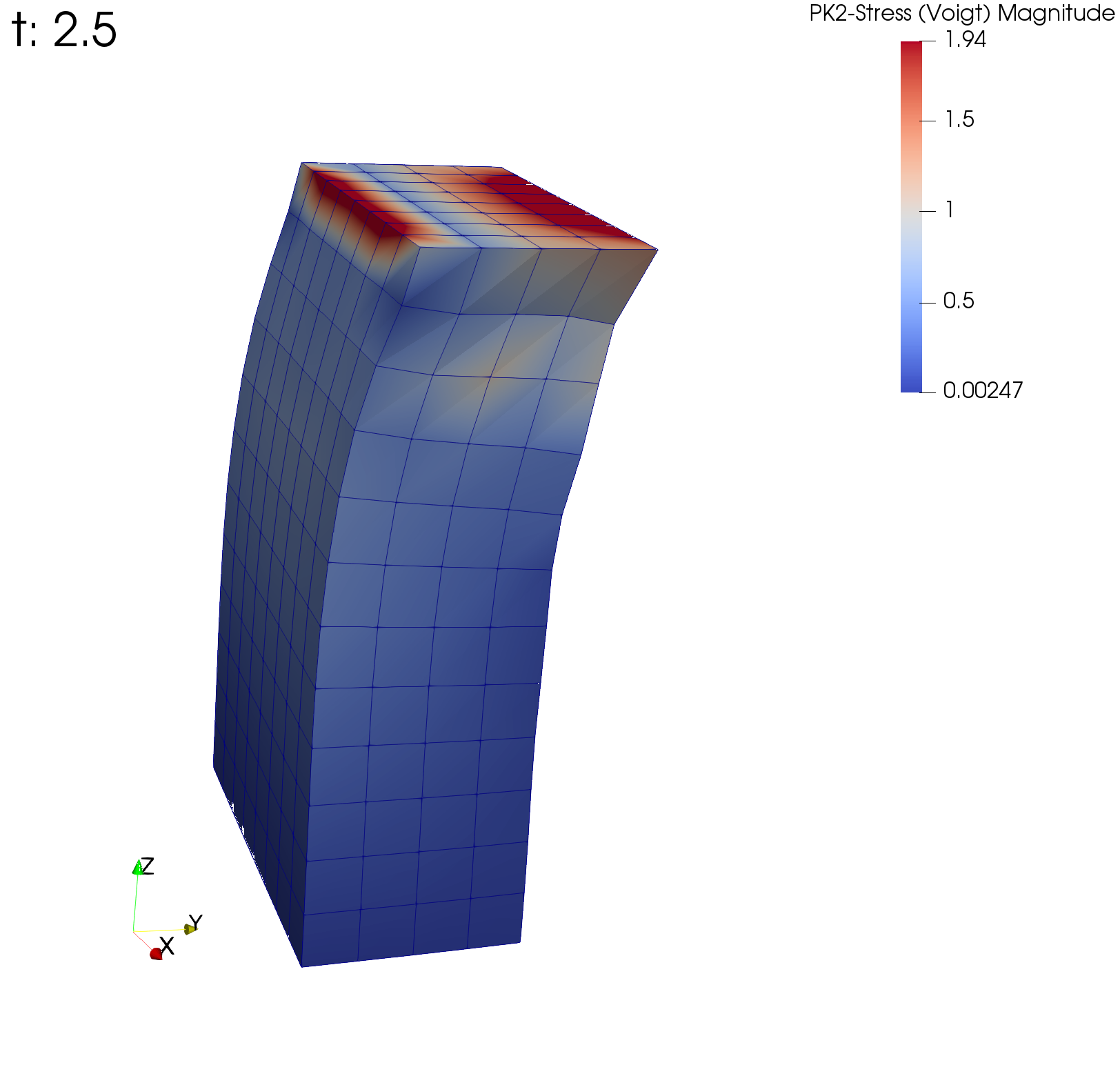
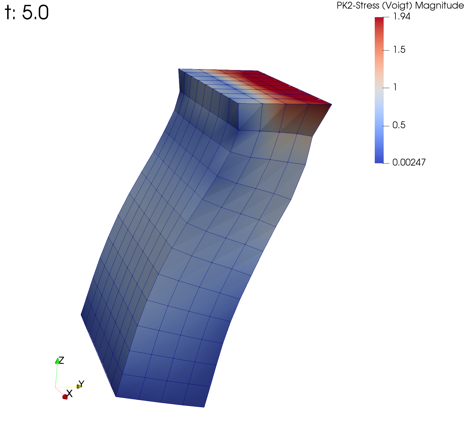
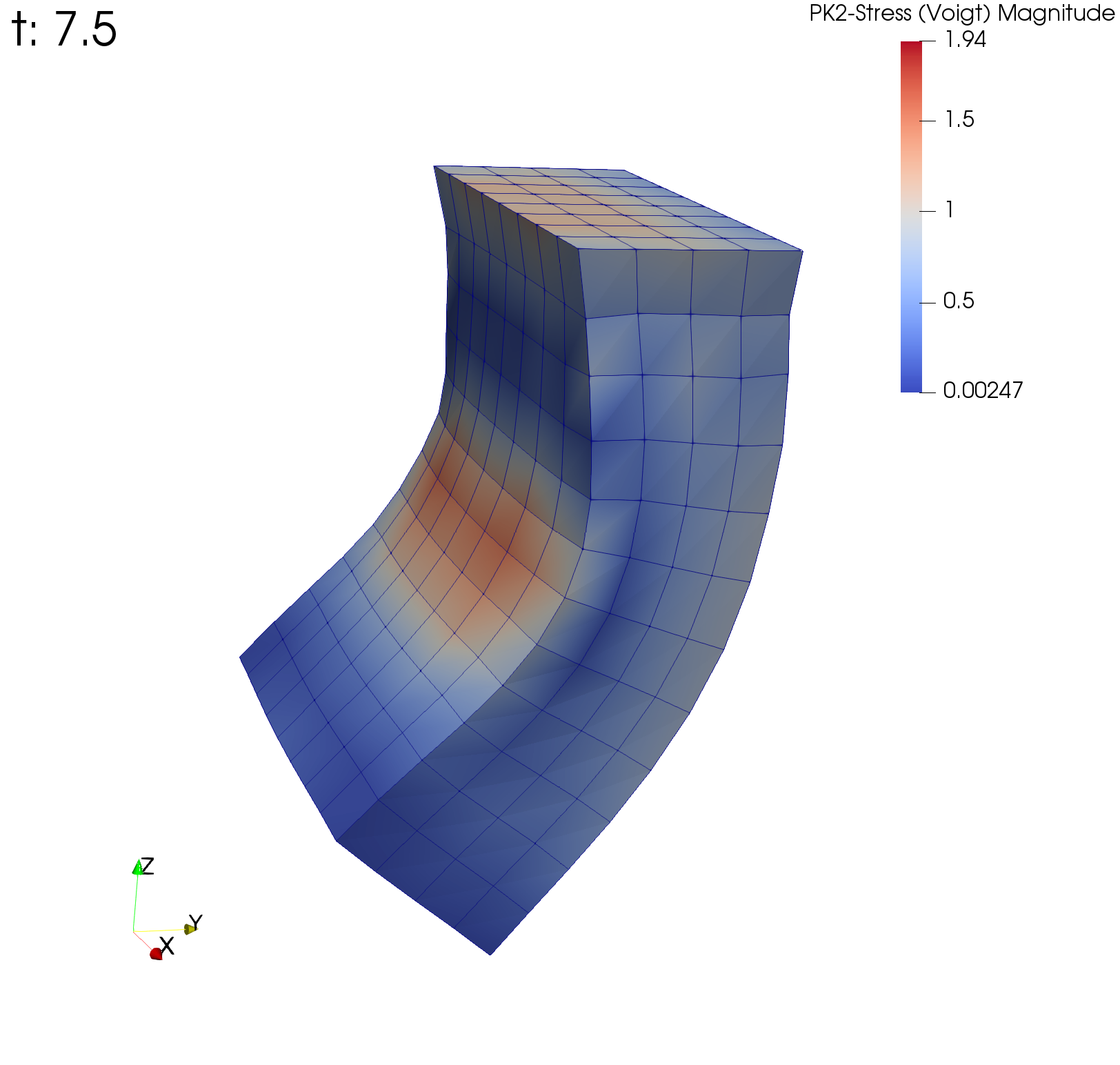
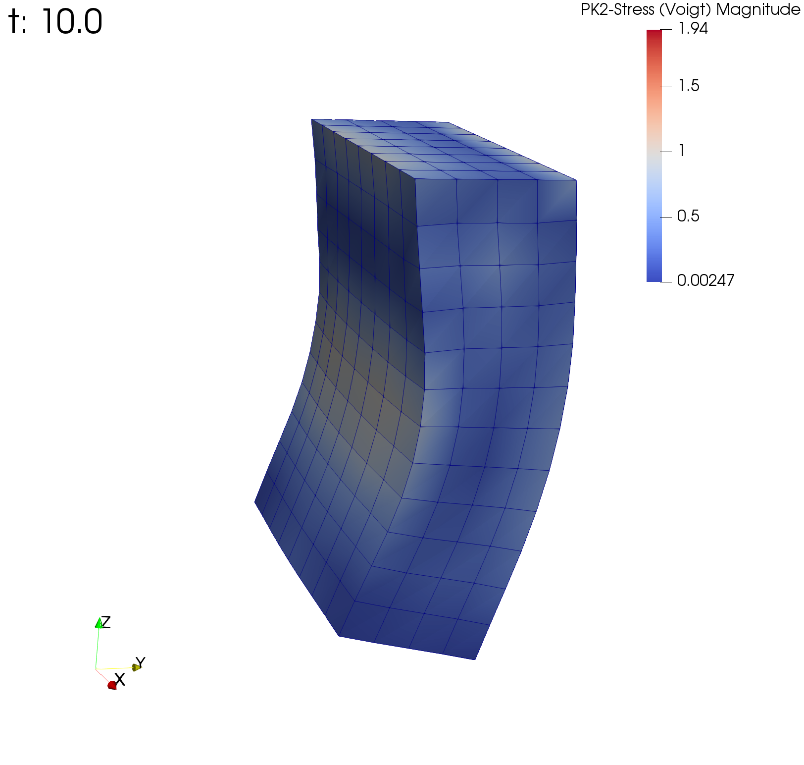
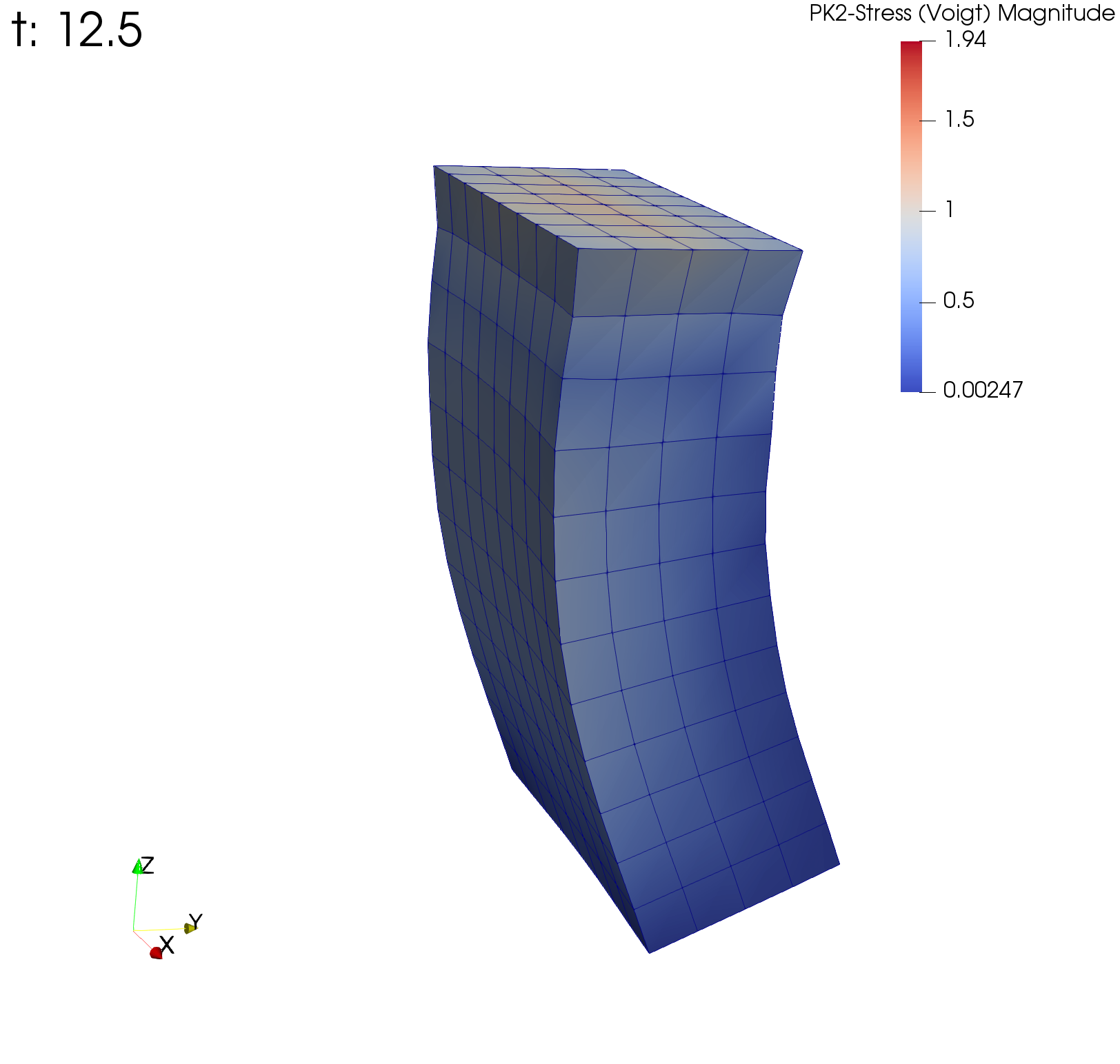
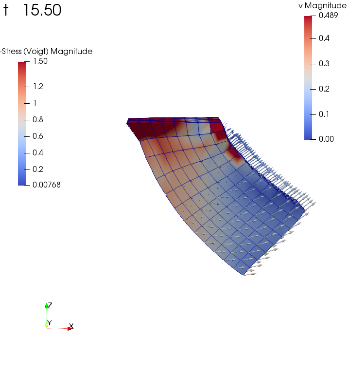
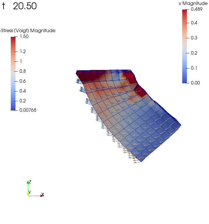
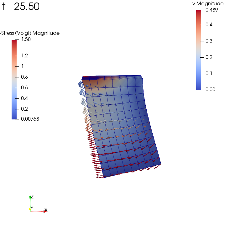
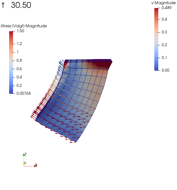
Scenario (3): A piece of gelatine moves from a varying force, this time in the longer direction of the hexaeder. This is realized with a traction force on the bottom that changes according to a sin function. This is a Neumann boundary condition that gets updated over time by a python callback function. The arrows visualize the current velocity vectors.
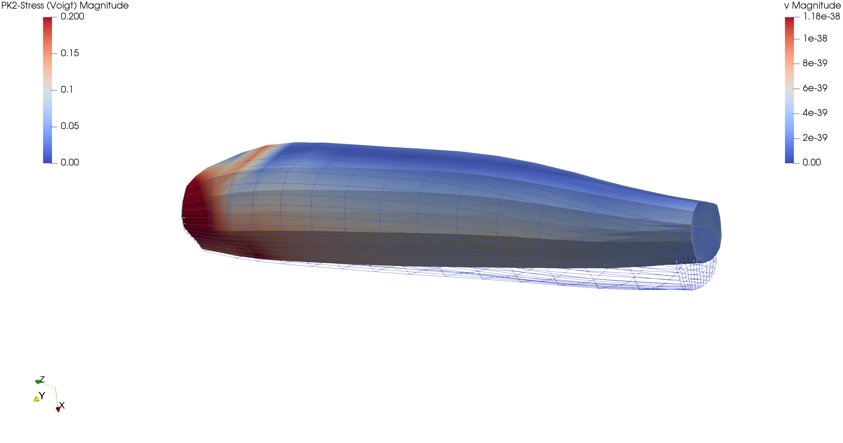
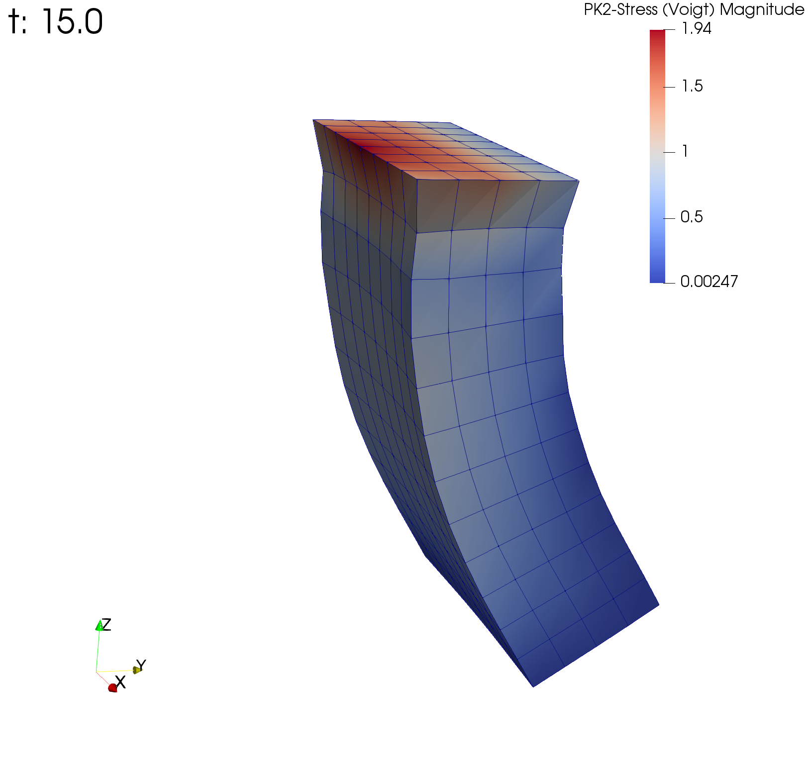
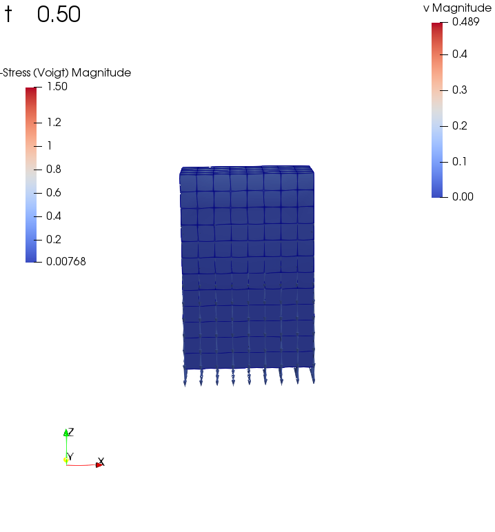
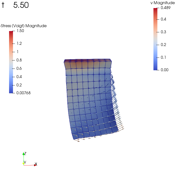
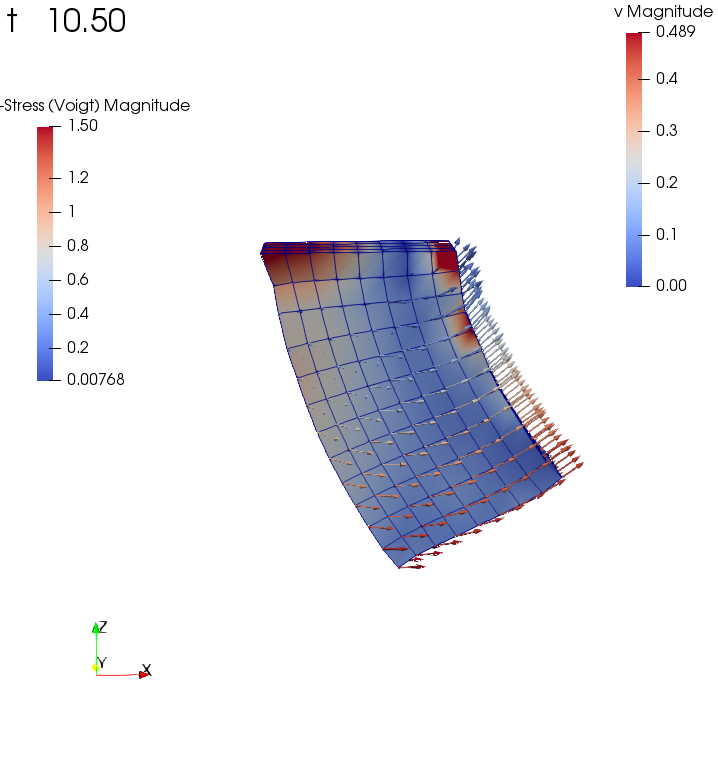
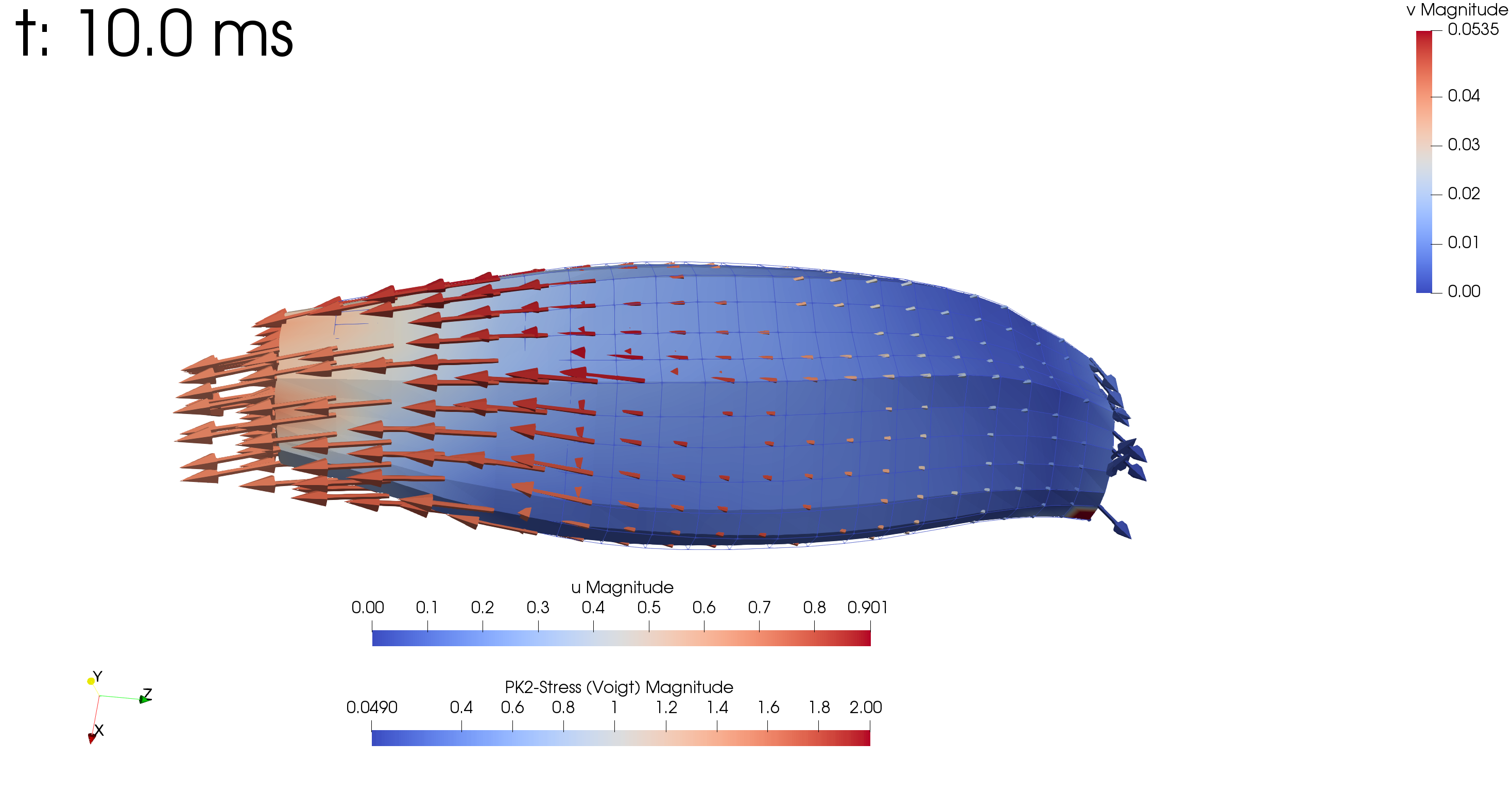
Fig. 32 Scenario (4): Dynamic simulation of muscle without active stress. The arrows indicate the velocity, colorung of the muscle volume is the 2nd Piola-Kirchhoff stress.
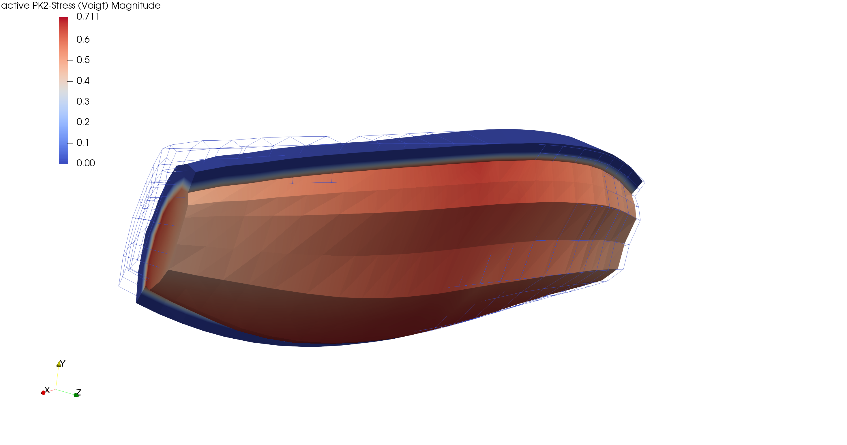
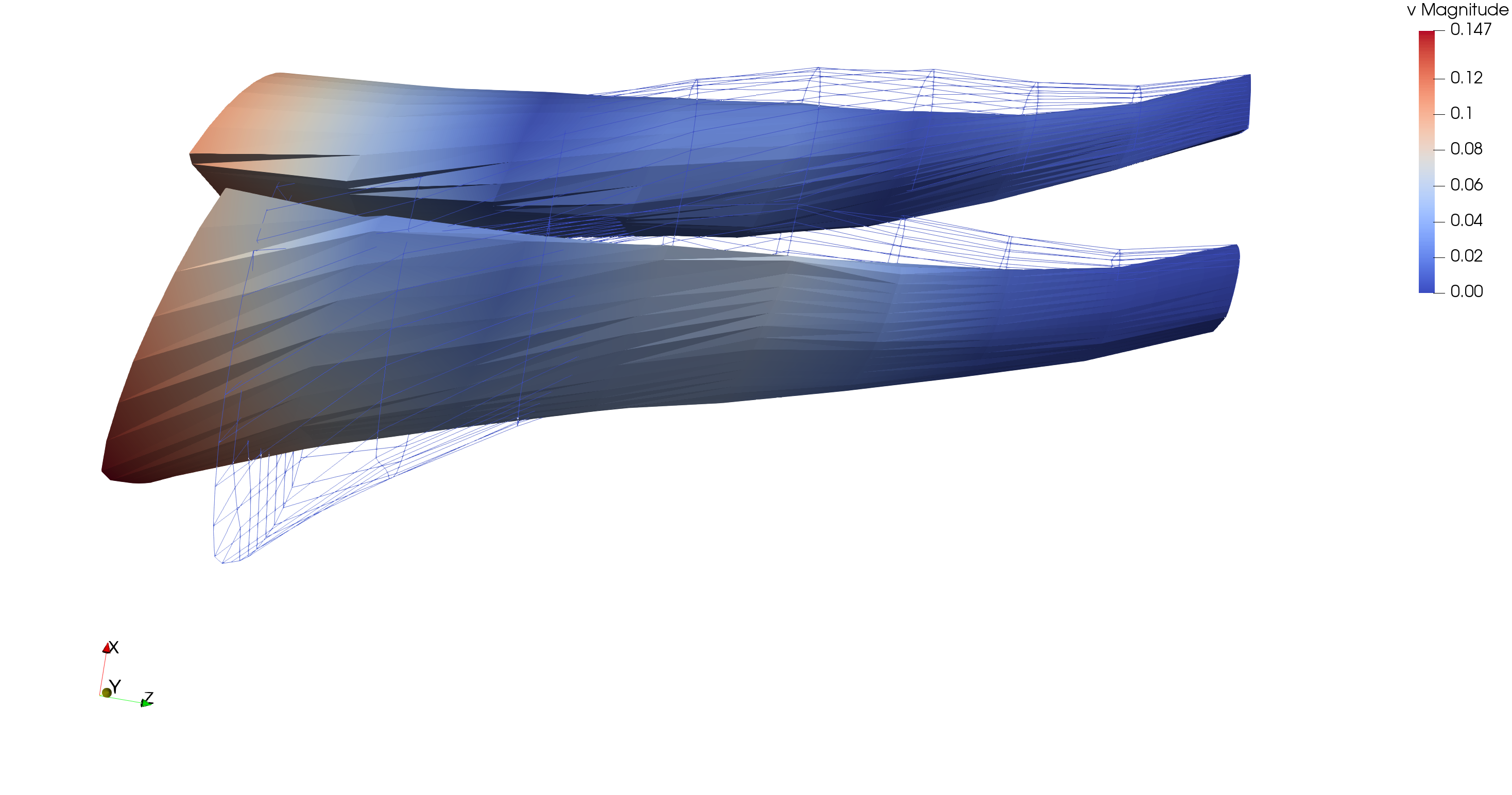
Fig. 33 Scenario (5): Dynamic simulation of muscle with fat layer, active stress is prescribed in the muscle domain.
This is a template example that shows how a custom material, given by its strain energy function, can be used.
The material can be defined in the C++ source file.
The first scenario is static the second is dynamic. It can also be run in parallel by prepending e.g. mpirun -n 2.
How to specify the material is described in Specification of the strain energy function.
This example uses FEBio to compute deformation of a Mooney-Rivlin material.
The same scenario is also simulated with opendihu and the results are compared.
This example needs FEBio installed. More specifically, you need to ensure that febio3 runs the febio executable
After running both programs (./febio and ./opendihu) there should be an output like
rms:2.5842881150700362e-06
This is the root mean square error between both results. If it is small like this, the results match.
If you get a message Error:Runningfebiofailedwitherrorcode256, then febio is not installed or something failed with febio.
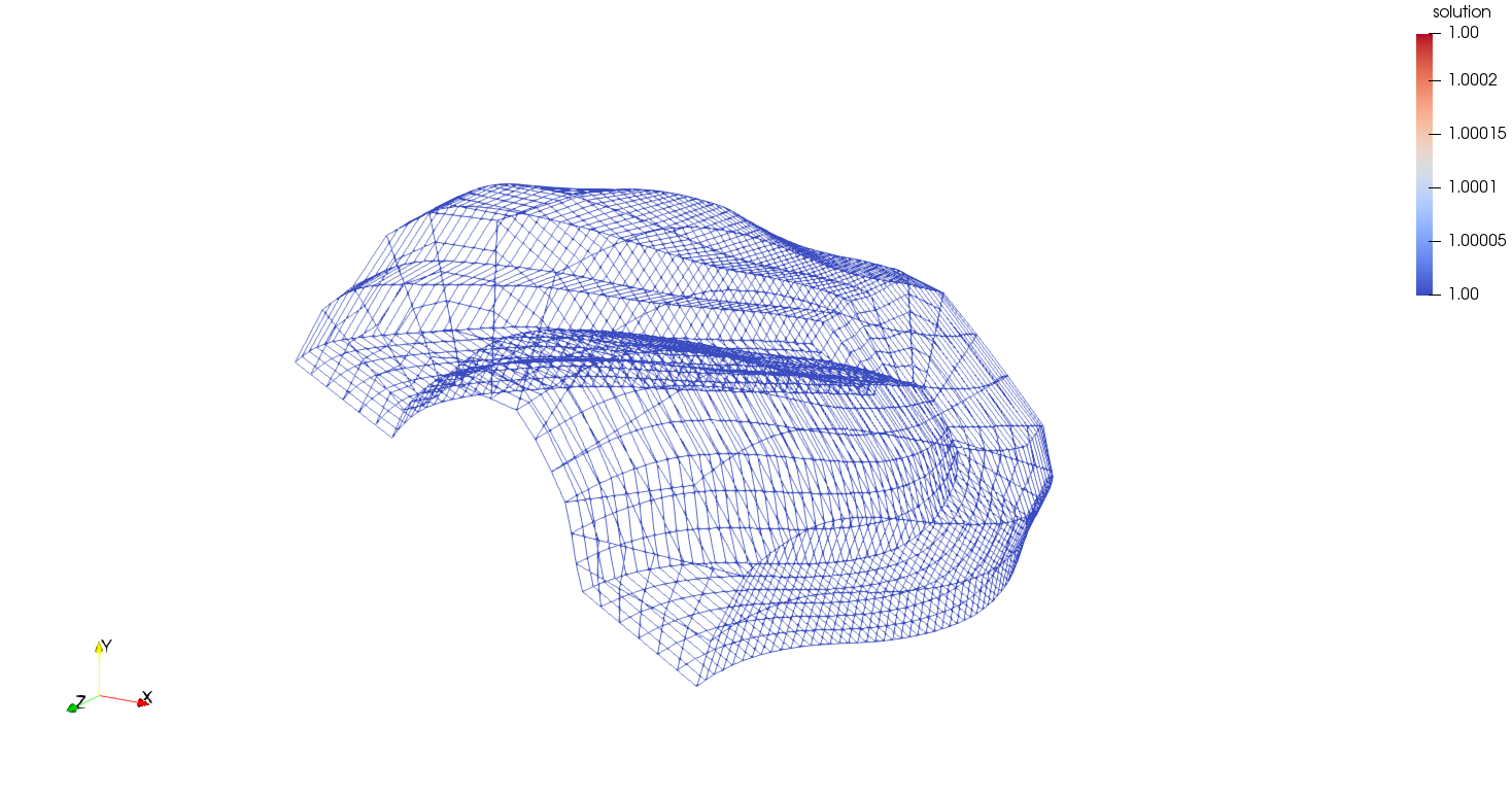
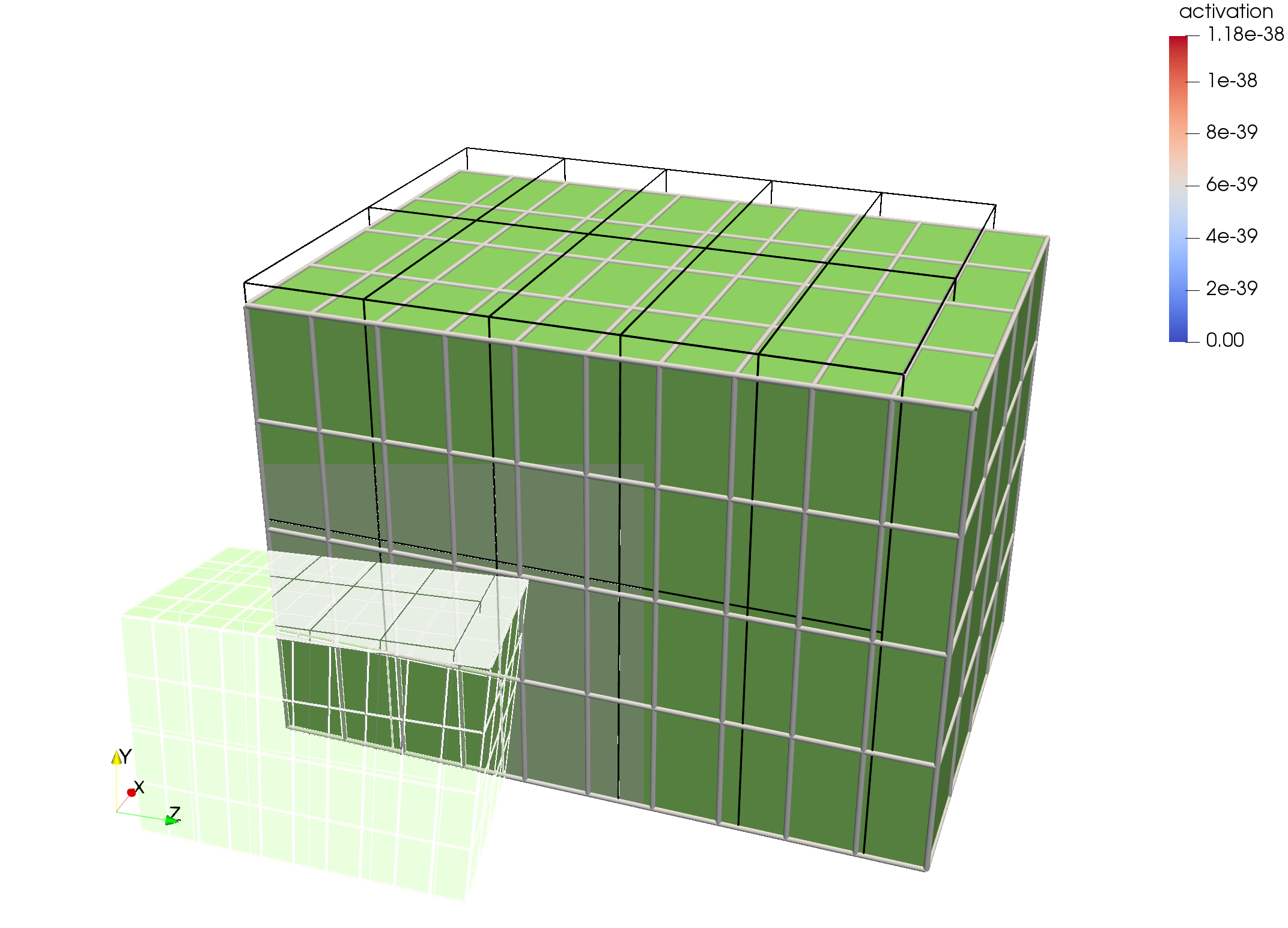
Fig. 36 Scenario for comparison of the results of FEBio and opendihu: The initial block (black lines) is extended to the right by a force. The result of opendihu is visualized by white tubes, the result of FEBio is visualized by the green solid. The results match.
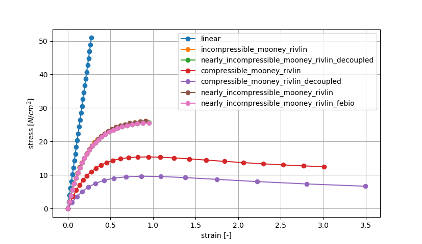
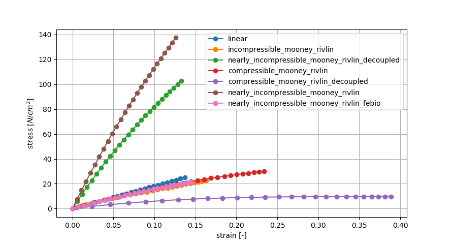
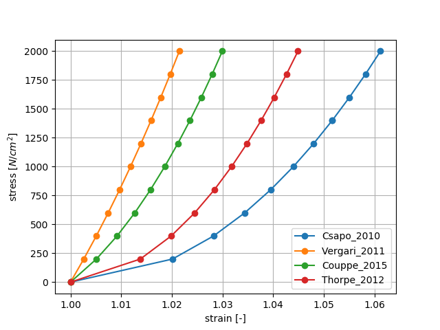
This example simulates a tensile test, where a block is extended uniaxially. The results for different materials are compared, also the same material with FEBio and opendihu.
Fig. 37 Result of the tensile test, stress-strain curves for different materials. It can be seen that for the incompressible material all the curves of the different formulations in opendihu and the curve for FEBio match and therefore the opendihu implementation is validated. The two compressible formulations cannot be compared because they have different parameters.
This example is for testing the Chaste integration in opendihu. It uses the hyperelasticity implementation of chaste if chaste has been installed.
It solves the nonlinear finite elasticity problem with Mooney-Rivlin material, for either 2D or 3D.
Because Chaste is not able to solve nonlinear elasticity in parallel, nor solve anything else than the quasi-static case,
integration in opendihu is not complete. This example is left here only if in the future someone wants to work on the chaste integration. Apart from that there is no use for Chaste.
In the core code it is only the QuasiStaticNonlinearElasticitySolverChaste that needs to be deleted.
Used by Thomas Heidlauf with OpenCMISS (scenario 4, “Titin”) and in the paper Heidlauf (2016) “A multi-scale continuum model of skeletal muscle mechanics predicting force enhancement based on actin–titin interaction”
contained environments: Aliev_Panfilov, Razumova
couples Aliev_Panfilov/I_HH, Razumova/l_hs and Razumova/rel_velo
computes active stress: Razumova/ActiveStress, the active stress is already multiplied by a force-velocity relation function \(f_\ell(l_\text{hs}) = f_\ell(\lambda_f)\).
9 states and 8 algebraics
Other models:
hodgkin_huxley_1952.cellml
The classical hodgkin huxley model with potassium channel and 2 sodium channels. This is sufficient for action potential propagation.
contained environments: razumova, sternrios, wal_environment, i.e. the Shorten model
computes razumova/activation and razumova/active_stress, the active stress is already multiplied by a force-velocity relation function \(f_\ell(l_\text{hs}) = f_\ell(\lambda_f)\).
Has inputs razumova/l_hs (fiber stretch) and razumova/velocity (contraction velocity).
This is a combination of the membrane model of Hodgkin-Huxley and the rest from Shorten. The rational is to have fatigue of Shorten but to make it faster using the simple Hodgkin-Huxley model for the membrane.
There are earlier versions that only differ in the initial values. This file has the correct initial values that are close to the equilibrium state.
computes razumova/activation and razumova/active_stress, the active stress is already multiplied by a force-velocity relation function \(f_\ell(l_\text{hs}) = f_\ell(\lambda_f)\).
Has inputs razumova/l_hs (fiber stretch) and razumova/velocity (contraction velocity).
44 states and 19 algebraics
hodgkin_huxley-razumova.cellml
This is a CellML model that computes activation and active stress values with only 9 states and 19 algebraics.
computes Razumova/activation and Razumova/active_stress, the active stress is already multiplied by a force-velocity relation function \(f_\ell(l_\text{hs}) = f_\ell(\lambda_f)\).
Has input Razumova/l_hs (fiber stretch) and Razumova/rel_velo (contraction velocity).
9 states and 19 algebraics
Notes for the connections with the continuum mechanical model:
Most CellML models compute an active stress that already has been multiplied by a force-velocity relation function \(f_\ell(l_\text{hs}) = f_\ell(\lambda_f)\). This is done using the variable l_hs which is an input to the model. However, the structure as described in Heidlauf2013 is such that the CellML outputs the factor \(\gamma \in [0,1]\) which gets multiplied by \(f_\ell(\lambda_f)\) in the mechanics solver.
In OpenCMISS, there was no scaling in the mechanics solver and, therefore, it had to be in the CellML model. With OpenDiHu, both ways are possible:
If the force-length relation should be considered in OpenDiHu and the mechanics solver, set “enableForceLengthRelation”: True and do not connect l_hs in the CellML model. Then, \(l_{hs}=1 \Rightarrow f_\ell(l_\text{hs})=1\). OpenDiHu implements the quadratic equation of Heidlauf2013.
If the force-length relation should be considered in the CellML model, set “enableForceLengthRelation”: False and connect the l_hs slot to the lambda output of the mechanics solver. This might be less efficient, because now lambda has to be transferred from opendihu to cellml, however it gives more flexibility because the force-length relation can be specified in the CellML model.
The reverse connection from the mechanics solver to the subcellular model usually includes the contraction velocity or shortening velocity. Opendihu computes the derivative of the fiber stretch, \(\dot{\lambda}_f\). This is a unit-less quantity. The CellML models need a value in micrometers per millisecond. The output of Opendihu can be scaled by the factor in option “lambdaDotScalingFactor” which is 1 by default. Some CellML models already do this scaling (those with rel_velo), then no rescaling is needed in opendihu.
The directory examples/electrophysiology/cellml contains example that solve a single instance of a CellML model, i.e. the same thing that OpenCOR does.
A CellML model is a differential-algebraic system (DAE) stored in an XML-based description language. The CellMLAdapter provides the following formulation:
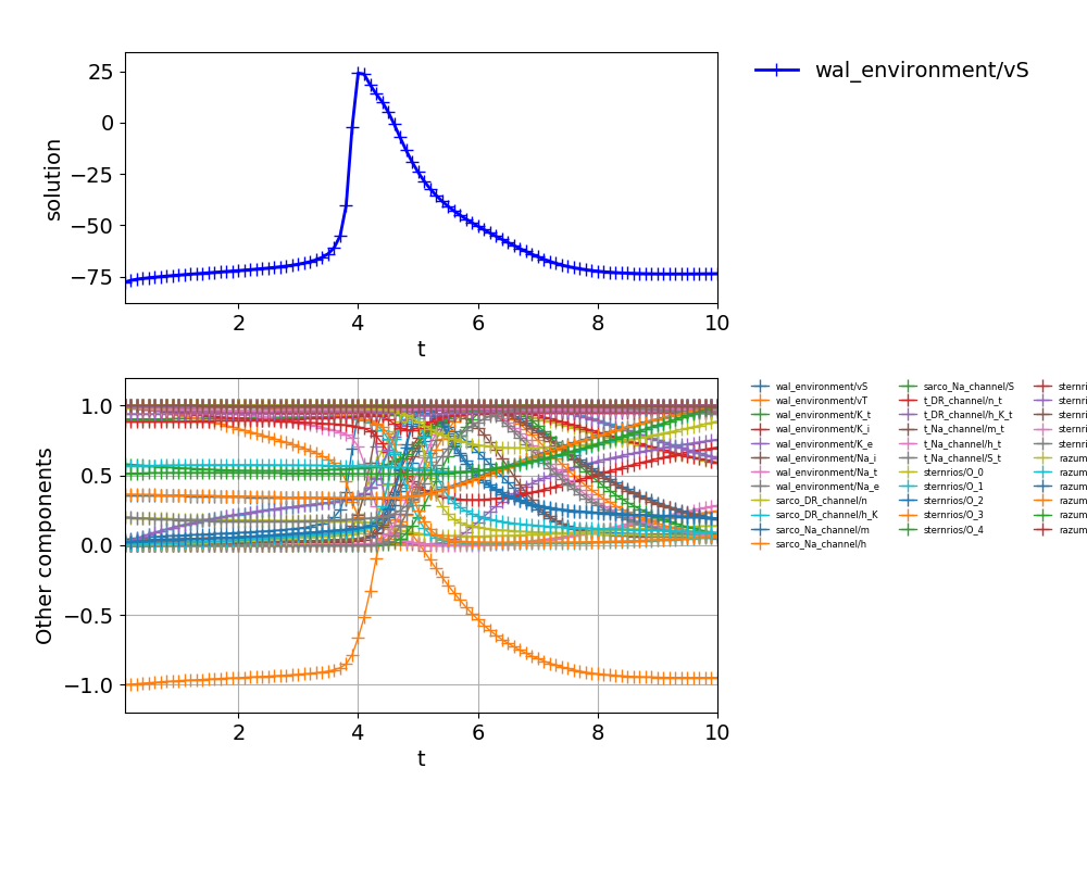
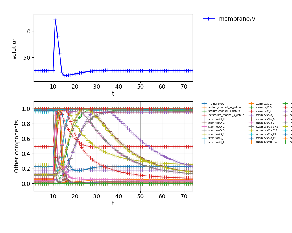
Simulates a single instance of the Shorten 2007 problem for 10s. It is stimulated at time 0.0. Plots values of Vm and gamma in out.png.
Note, this uses a very fine timestep width of 1e-5 and explicit integration. This is only for debugging and demonstration, you
can replace the ExplicitEuler by, e.g., Heun integration
Fig. 42 Models for the examples with Monodomain equation.
The Monodomain equation describes action potential propagation on a muscle fiber. It can be derived from modeling the intra and extracellular space and the membrane as an electric circuit. It is given by
\(V_m\) is the trans-membrane voltage, i.e. the voltage between intracellular and extracellular space,
\(A_m\) is the fibers surface to volume ratio,
\(C_m\) is the capacitance of the fiber membrane,
\(\sigma_\text{eff}\) is the scalar effective conductivity of the system that can be computed from the intra and extracellular conductivities, \(\sigma_\text{in}\) and \(\sigma_\text{ex}\) as \(\sigma_\text{eff} = \sigma_\text{in} \parallel \sigma_\text{ex} = (\sigma_\text{in} \cdot \sigma_\text{ex}) / (\sigma_\text{in} + \sigma_\text{ex})\)
\(I_\text{stim}\) is an external stimulation current that models the external stimulation from the neuromuscular junction.
\(\textbf{y}\) is a vector of additional states that are solved by a system of ODEs. The states correspond to ion channels in the membrane. Different formulations are possible for this ODE system.
This solves the Monodomain equation with the classical subcellular model of Hodgkin and Huxley (1952).
It is used to demonstrate several things about the Monodomain solver and nested solvers in general (because this is the easiest example, were a :doc:/settings/splitting` scheme is used).
For plotting the result, cd into the out directory as usual. Now you can see that two types of Python files have been created: some starting with cellml_ and other starting with vm_. Only plot either of them, e.g. with plotcellml_00000* or plotvm*.
If you look into the settings, you’ll see that the cellml files were written by the CellmlAdapter and therefore contain all state variables. The vm files were created by the Timestepping scheme of the diffusion solver and, thus, contain only the solution variable of the diffusion solver, i.e., the transmembrane-voltage.
Because the option "nAdditionalFieldVariables" is set to 2, also values of the two additional field variables will be written to the vm files. These field variables get values of the gating variables m and h of the membrane model. This is done by connecting their Connector Slots, as can be seen in the solver structure visualization.
A reason for maybe not wanting to output the variables directly in the CellmlAdapter is that those files contain a lot of data and this will be time consuming for more advanced examples. Then, only writing the files with the variable of the diffusion is a good option.
Now the threre existing mechanisms to connect data slots are outlined.
The first mechanism to connect slots is by naming the slots the same, then they are automatically connected and the data is transferred. This is done with the m variable in this example.
The second mechanism is to specify the connections in the global setting “connectedSlots”. This is done for the h gating variable, as follows:
config={..."connectedSlots":[("h","h_gate"),# connect the additional field variable in the output writer("h_gate","h"),],...
Here, the two slots h_gate and h are connected, h_gate is the name of the slot at the CellmlAdapter and h is the slot name at the additional field variable, directly at the output writer.
There is a third mechanism to connect two slots: by specifying the connection in the splitting scheme under the options "connectedSlotsTerm1To2" and "connectedSlotsTerm2To1". This is also done here for connecting the transmembrane voltage, \(V_m\), between the CellmlAdapter and the diffusion solver.
When running
plotcellml_00000*
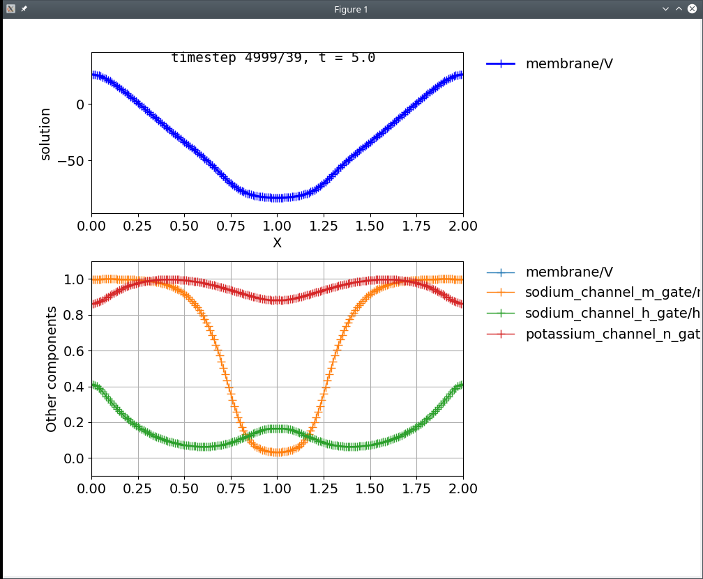
in the out folder, you get the following animation:
Fig. 43 This shows the propagation of an action potential (here a snapshot at a given point in time, run the plot script to see the animation).
Command (1) uses the FastMonodomainSolver and takes 4 seconds. Command (2) does not use the FastMonodomainSolver and takes 17 seconds.
To check that both compute the same results there is a script cmp.py in the build_release/out directory. After compilation, run the following commands in the build_release directory:
rm-rfout/fastout/not_fast
./not_fast_fiber../settings_fast_fiber.py# this outputs to directory `fast`
mvout/fastout/not_fast# rename output to `not_fast`
./fast_fiber../settings_fast_fiber.py# this again outputs to `fast`# now we have results from `fast_fibers` in directory `out/fast`# and results from `not_fast_fibers` in directory `out/not_fast`cdout
./cmp.py
As can be seen the final average error is quite big. From the individual errors of the files we can see that the error gets bigger over time. This is the result of the stimuli occuring to slightly different times, which leads to higher error values.
You can also plot the results in the out/fast and out/not_fast directories and see that they match qualitatively. Both results contain 10 stimuli.
This example uses a motoneuron model to schedule the stimuli, whereas in the previous examples, the stimulation times were given by the settings. Then, the Monodomain equation is computed with the Hodgkin-Huxley subcellular model. This example also demonstrates how to use the MapDofs class in an approach without python callbacks.
This requires a prepared motor neuron model with input and output variables. The model used by this example is a modified Hodgkin-Huxley CellML model (motoneuron_hodgkin_huxley.cellml). This means there are two Hodgkin-Huxley models, one for the motor neuron and one for the Monodomain equation.
If an existing motor neuron CellML model should be used without modification, e.g. the normal Hodgkin-Huxley model, then a different approach with python callbacks would be needed.
How it works can be explained with an part from the solver_structure.txt file:
Here, vm is the field variable for the transmembrane voltage, \(V_m\), that is used in the Monodomain equation. At a given time, the first MapDofs call copies the values of vm from the center point of the fiber to the v_in slot, which is an input to the motor neuron model. If the motor neuron does not fire, it sets the output value v_out equal to the input value v_in. The CellML motor neuron model is also advanced in time and eventually depolarizes and “fires”. Then the v_out variable gets to value of 20. Then, the second MapDofs action copies the value of v_out back to vm at the 3 center nodes of the fiber. The new prescribed value leads to a stimulation at the center of the fiber.
The modifications needed in the CellML model are the threshold condition, that sets the output value v_out. The additional code in the CellML model of the motoneuron is as follows:
defcompfiring_thresholdasvar{membrane_V}V:millivolt{pub:in};varV_extern_in:dimensionless{init:-75};// input membrane voltage, from fibre sub-cellular modelvarV_extern_out:dimensionless;// output membrane voltage, to fibre sub-cellular modelvarV_threshold:millivolt{init:0};// threshold of V, when it is considered activevarV_firing:dimensionless{init:20};// constant value to which V_extern_out will be set when motoneuron firesV_extern_out=selcaseV>V_threshold:V_firing;otherwise:V_extern_in;endsel;enddef;
Use the following commands to compile and run the example.
The following subcellular models are also implemented. The examples are very similar to the hodgkin-huxley example except for the different CellML model file.
All of these examples run also in parallel and can be started by prepending, e.g., mpirun-n4.
motoneuron_cisi_kohn
This is again the normal Monodomain with subcellular model of Hodgkin-Huxley, but it uses the motor neuron model of Cisi and Kohn. This is an approach with a python callback function that does not need any modification of the CellML model in use. The callback function demonstrates how to delay a signal.
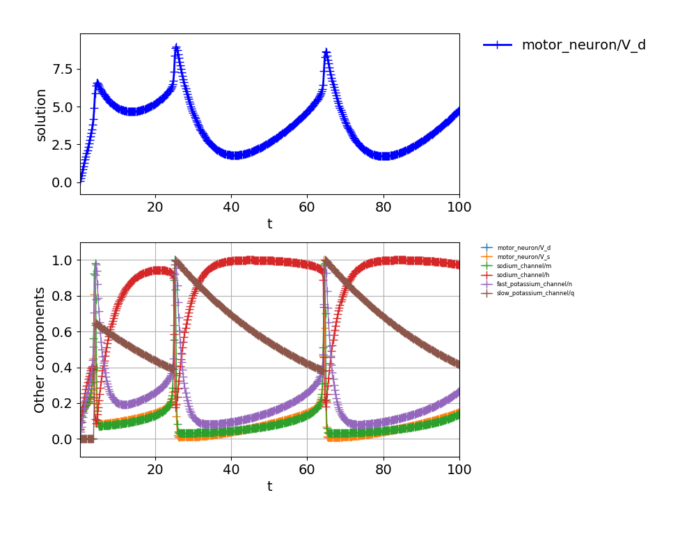
Fig. 45 This shows the evaluation of the motoneuron over time.
hodgkin_huxley-razumova
This is a CellML model that computes activation and active stress values with only 9 states and 19 algebraics. The example also directly outputs png files, so no additional plot command is required.
shorten_ocallaghan_davidson_soboleva_2007
This is the Shorten model, see the description here.
new_slow_TK_2014_12_08
This is the model that was used in OpenCMISS, it is a variant of the Shorten model.
The following examples all include fibers, where the Monodomain Equation is solved.
This can be done by either building the splitting scheme from nested solvers (e.g. as in multiple_fibers, multiple_fibers_cubes_partitioning, fibers_emg, cuboid) or by using the faster FastMonodomainSolver (e.g. in fibers_emg, fibers_fat_emg, fibers_contraction).
Multiple instances of the Monodomain equation, i.e. multiple biceps fibers with electrophysiology. The fibers are not subdivided to several subdomains.
When using multiple processes, every process simulates whole fibers. The example has an easy settings file that contains all configuration in a single file.
Fig. 46 Models that are used in the multiple_fibers example.
This example has MegaMol integration but also outputs Paraview files. If run without MegaMol enabled in opendihu, it will display an error, but work normally.
The number of fibers depends on the number of processes.
It is not possible with this example to have cube-shaped partitions because of the solver structure.
In order to have a process compute multiple fibers but only a part of them, use the multiple_fibers_cubes_partitioning example.
Compare multiple_fibers_cubes_partitioning/src/multiple_fibers.cpp with multiple_fibers/src/multiple_fibers.cpp to get the difference.
Again multiple fibers but this time they can be subdivided such that every process can compute a “cubic” subdomain that contains parts of several fibers.
The model is the same as in Fig. 46.
Multiple 1D fibers (monodomain), biceps geometry
This is similar to the fibers_emg example, but without EMG.
if fiber_file=cuboid.bin, it uses a small cuboid test example (Contrary to the “cuboid” example, this produces a real cuboid).
You can do the domain decomposition yourself or let the program decide it.
Doing in manually means setting the option n_subdomains. The given number of subdomains has to match the number of processes, e.g. 2x2x1 = 4 processes.
The domain decomposition can be specified in x,y and z direction, where the fibers are aligned with the z axis.
Examples:
--n_subdomains221, \(2\times 2\times 1\), this means no subdivision per fiber,
--n_subdomains884, every fiber will be subdivided to 4 processes and all fibers will be computed by 8x8 processes.
Example with 4 processes and end time 5, and otherwise default parameters:
Three files contribute to the settings:
A lot of variables are set by the helper.py script, the variables and their values are defined in variables.py and this file
creates the composite config that is needed by opendihu.
You can provide parameter values in a shorten.py file in the variables subfolder. (Instead of shorten.py you can choose any filename.)
This custom variables file should be the next argument on the command line after settings_fibers_emg.py, e.g.:
This is the main example for multiple fibers without fat layer. Again multiple fibers can be subdivided, furthermore everything is coupled to a static bidomain equation. This example was used for large-scale tests on Hazel Hen (supercomputer in Stuttgart until 2019) and was successfully executed for 270.000 fibers on 27.000 cores. (Same as Fig. 46)
Both scenarios, (1) and (2), compute the same, but (2) uses the FastMonodomainSolver and, thus, is by a factor of ~10 faster.
Any number of processes can be used, the partitioning is done automatically such that all processes are used and cube-shaped partitions are generated. Thus, it makes sense to provide a number of processes that has a lot of divisors, like 60.
The settings for this example consists of two files that are the two parameters to the command: the main file is settings_fibers_emg.py where all settings for
the solvers are specified.
Some of the values there have variables that are set in the second file. The second settings file in this example is ramp_emg.py.
The file is stored in the variables subdirectory.
It is more compact and contains only the values that need to be specified for a particular scenario.
If a simulation with a different set of parameters is needed, the best way is to create a copy of the scenario file in the variables directory and adjust it.
Then call the simulation with this filename as the second argument.
Additionally, there is a number of parameters that can be overwritten on the command line, for details see
Whereas all previous examples use biceps brachii geometry, this example is simply a cuboid
and does not need any geometry information at all. Only here, the number of nodes per fiber can be adjusted.
This example has a fixed number of fibers that are not at a specified geometry. (In fact, they are all on top of each other.)
The settings file is very short and contains all needed information. This is much simpler than the other electrophysiology examples.
The purpose of this example is to test numerical parameters or do performance measurements where a specific number of fibers and processes is needed.
The Monodomain equation is solved with the shorten subcellular model. (The same as in Fig. 46)
You have to pass additional arguments to the program:
# arguments: <n_processes_per_fiber> <n_fibers> <n_nodes_per_fiber> <scenario_name># scenario with 2 fibers with 100 nodes each (1):
./cuboid../settings_cuboid.py12100test_run
# 2 fibers with 2 processes each, i.e. 4 processes in total (2):
mpirun-n4./cuboid../settings_cuboid.py22100parallel
# 4 fibers with 2 processes each, i.e. 8 processes in total (3):
mpirun-n8./cuboid../settings_cuboid.py24100test
The number of processes per fiber times the number of fibers has to be equal to the given number of processes in mpirun.
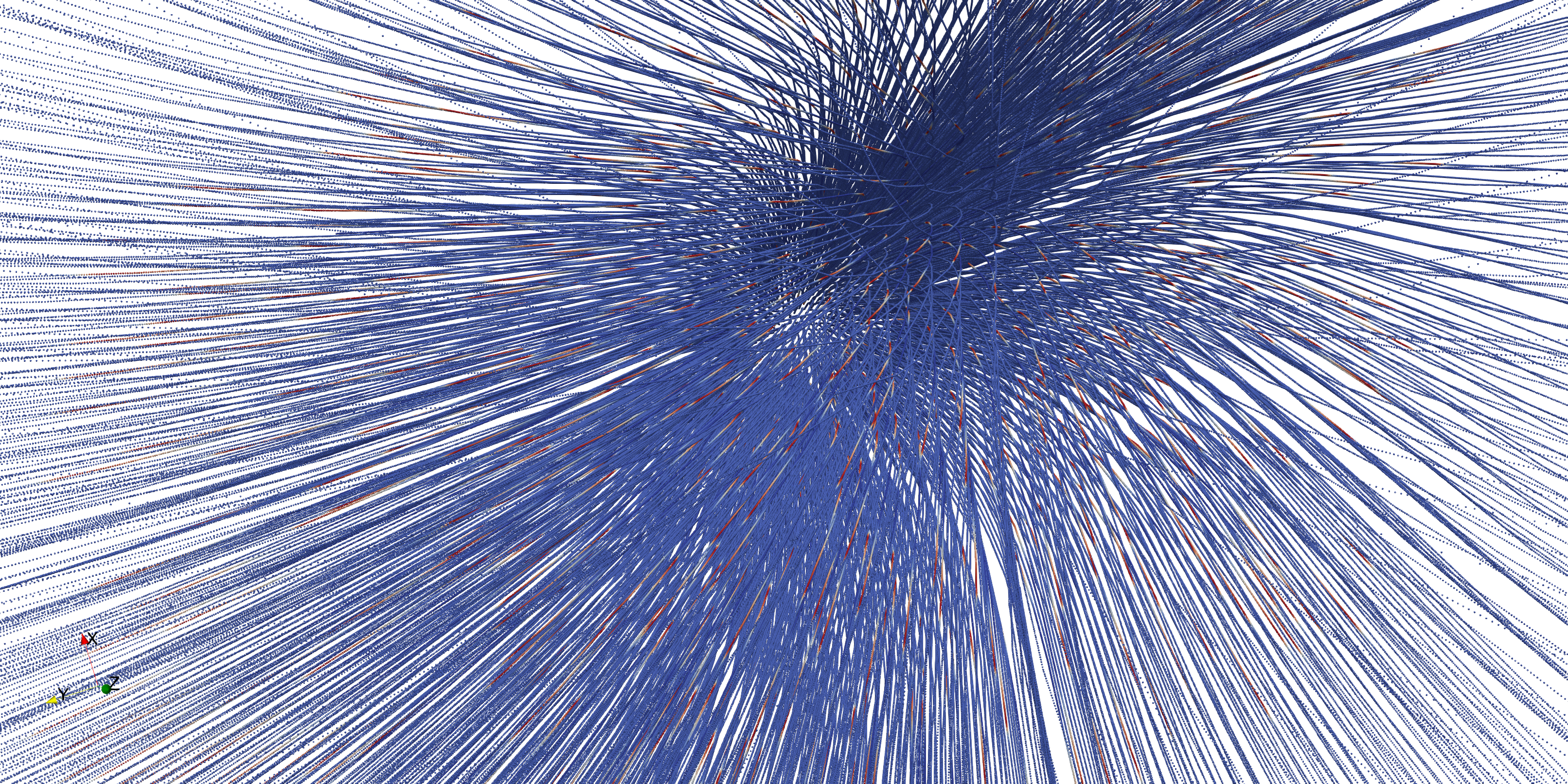
Fig. 50 This shows how the fibers are aligned spatially (for scenario (2)), click to enlarge.
This example adds a fat and skin layer to simulate EMG signals on the skin surface. It is also configured to sample signals at a simulated high-density EMG electrode array on the skin surface.
The data is written to a VTK and a csv file.
Fig. 51 Models that are used in the fibers_fat_emg example.
The example can be compiled and run by the following commands. Instead of 2 processes, more are possible and often beneficial, depending on the used computer. This examples has very good parallel scaling.
Similar to fibers_emg, The settings for this example consists of two files that are the two parameters to the command: the main file is settings_fibers_fat_emg.py where all settings for the solvers are specified.
Some of the values there have variables that are set in the second file. The second settings file in this example is biceps.py. The file is stored in the variables subdirectory.
It is more compact and contains only the values that need to be specified for a particular scenario.
If a simulation with a different set of parameters is needed, the best way is to create a copy of the scenario file in the variables directory and set adjust it. Then call the simulation with this filename as the second argument.
Additionally, there is a number of parameters that can be overwritten on the command line, for details see
The results are written to several files in the out/<scenario> directory, e.g. out/biceps.
There are different files containing fibers, the muscle and fat volume, only the surface and the electrodes. The intervals in which these files are written can be adjusted in the scenario file.
The fibers and volume files have a large size, whereas the surface and electrode files have small sizes. When running simulations with long time spans or high resolution, output storage can be a problem.
Then, it makes sense to only output surface and electrode data, as this is usually the interesting data.
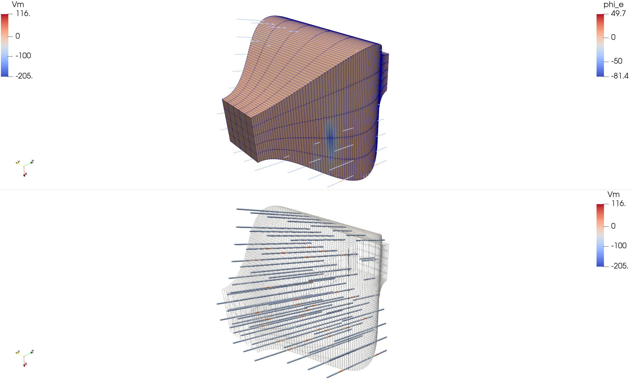
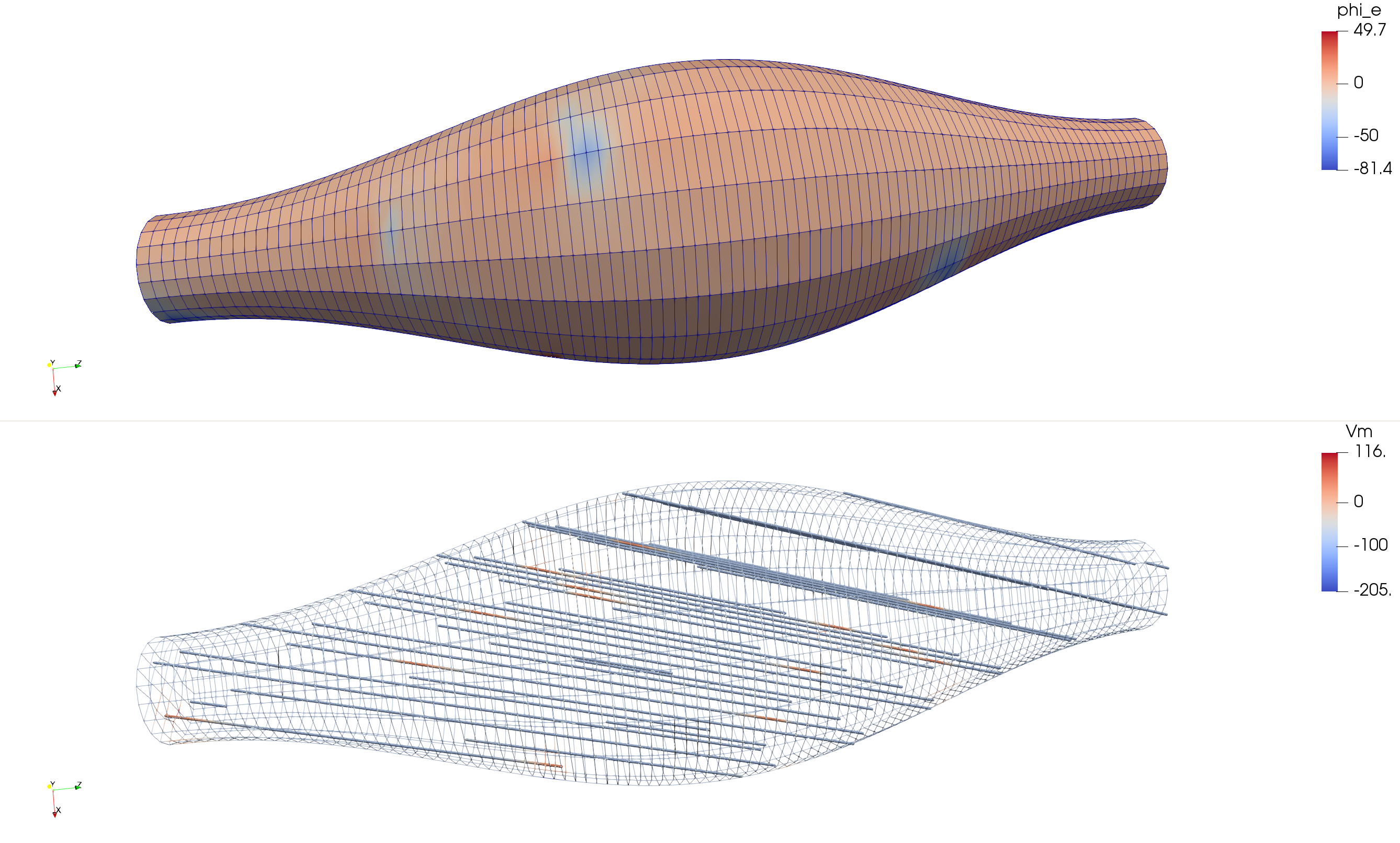
Fig. 52 Top: Fibers and surface, bottom: volume of muscle and fat.
Fig. 53 Electrodes with EMG values. The values are the same as in the surface.
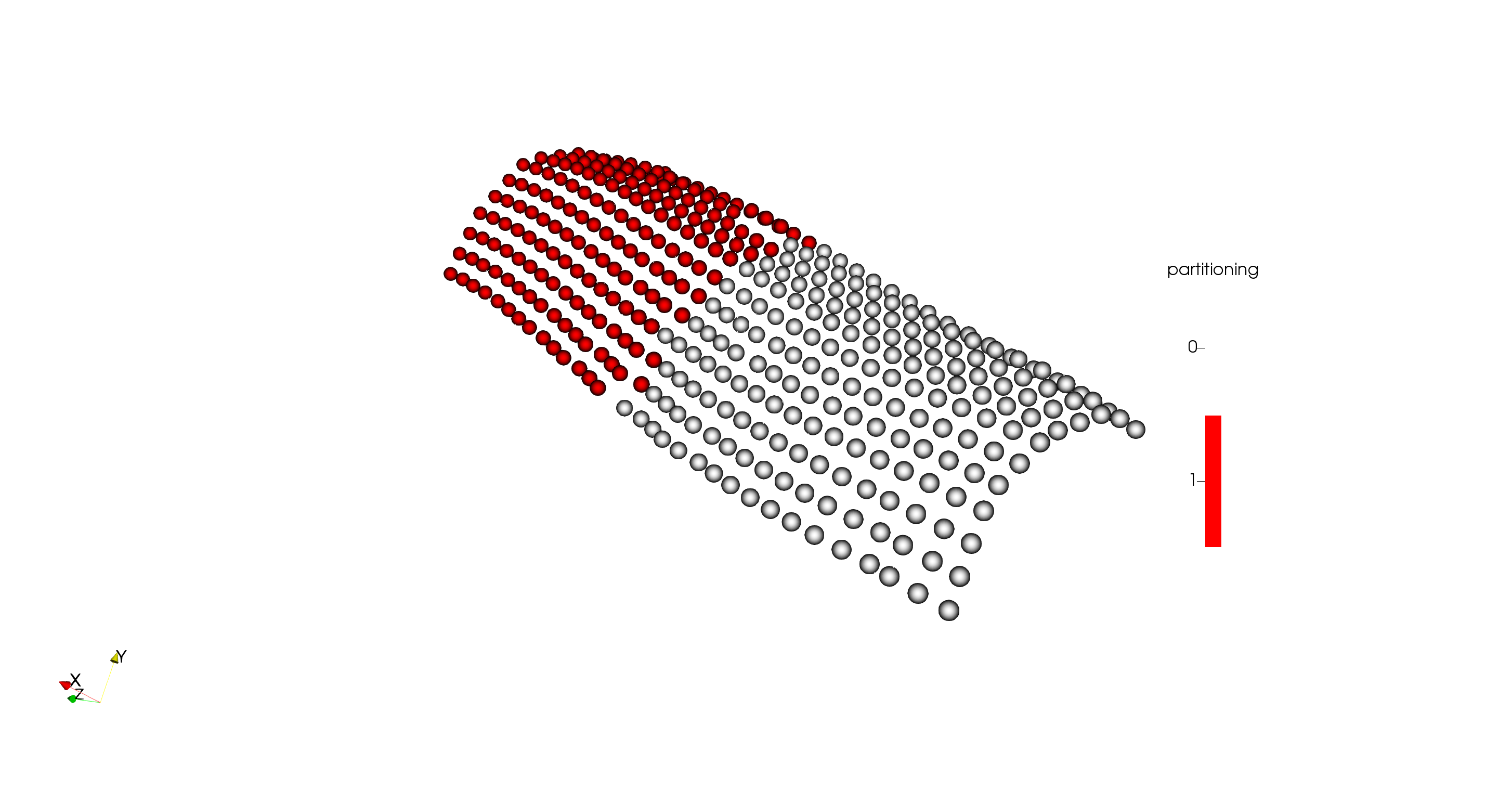
Fig. 54 Surface electrodes with the process number for the example of two processes. It can be seen how the domain is split to rank 0 and 1. The EMG values are only computed on their respective rank.
For the surface output files, each rank writes their own data, i.e. there is no communication of data between the ranks for the output (which is efficient). For the electrode values, all values are send to rank 0 which writes the data to a file.
This is still acceptible because the number of electrodes is usually small compared to the resolution of the 2D and 3D meshes.
Initially, each process tries to find as many of the electrode points as possible on its own subdomain. Which points are found by which rank can be seen by the electrodes_found* and electrodes_not_found files.
Some points will be found by multiple processes. Then only the values on the rank that actually own the subdomains are used.
The electrode data is always written in two formats. First, for ParaView (*.vtp), second as CSV file.
The csv files are for easier processing with other tools or python scripts. The csv file is called electrodes.csv.
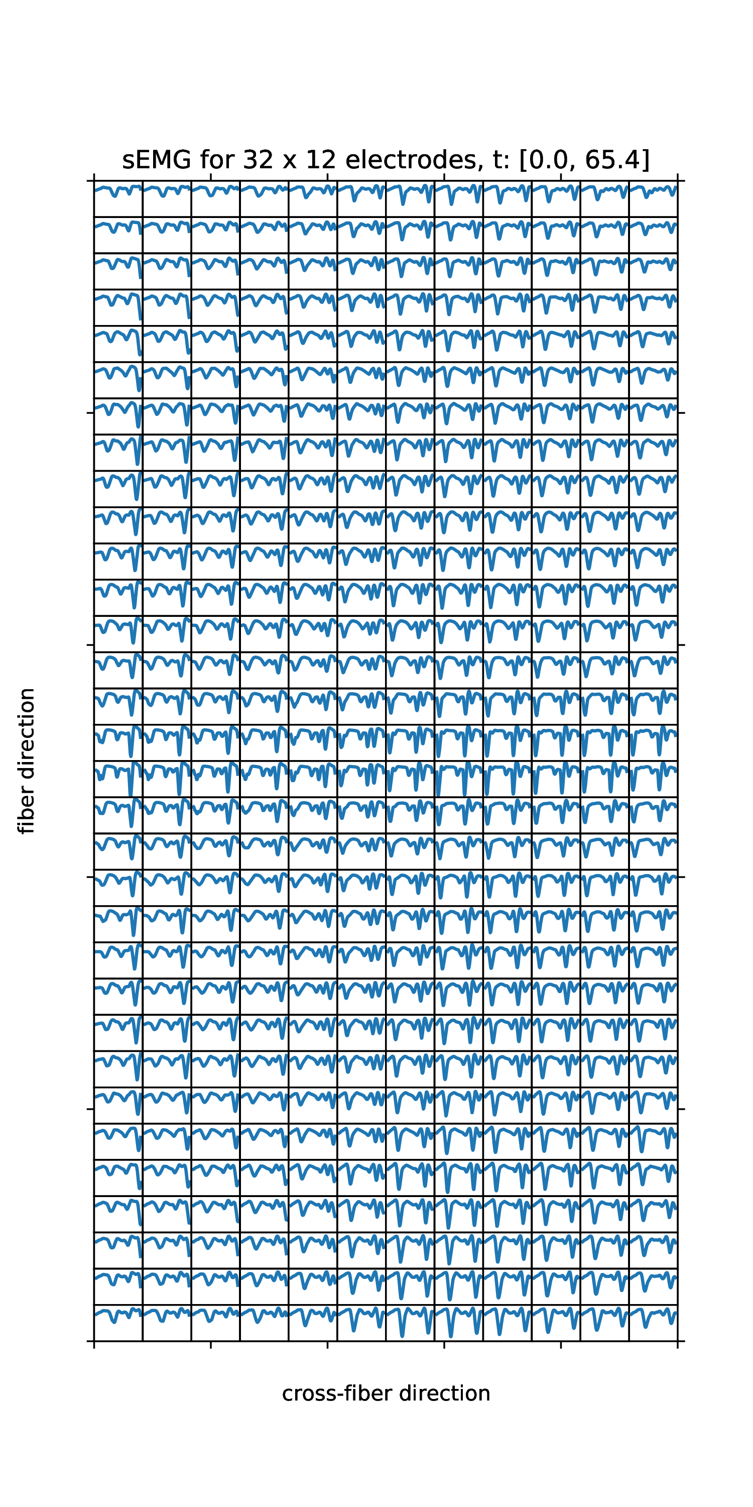
There is one script that visualizes all EMG measurements over time. It is located in the top level directory of the exercise.
cd$OPENDIHU_HOME/examples/electrophysiology/fibers/fibers_fat_emg
./plot_emg.py# use the default file
./plot_emg.pybuild_release/out/biceps/electrodes.csv# specify the file manually
This example uses an analytical description of action potential propagation, which replaces the Monodomain Equation on the fibers. Multiple fibers are coupled with Bidomain equation.
Thus, this example is the same as fibers_emg, except that Monodomain eq. is replaced by an analytic equation.
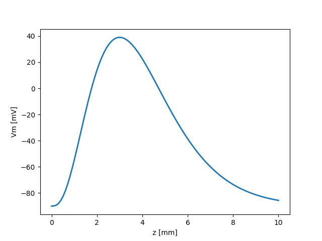
\[\begin{split}G(z) = \begin{cases}
96\,z^3\,exp(-z) - 90 & \text{ for } z \geq 0 \\
-90 & \text{ for } z < 0
\end{cases}\end{split}\]
where \(z=U\cdot t\) with propagation velocity \(U\), see Fig. 55.
Fig. 55 Rosenfalck function \(g(z)\). Note the the shapes of the propagating stimuli correspond to this graph, propagating to the left (negative z axis).
Szenario (1) uses the biceps geometry and fiber files. It can be run in parallel.
Scenarios (2) and (3) use a custom geometry that is defined in the python settings. The fibers are independent of the muscle geometry and can be parametrized with different angles. These scenarios only run in serial.
Fig. 57 Results of scenario (2). The geometry has a square cross-section of the muscle. The “radius” along the muscle follows a sine curve.
Fig. 58 Results of scenario (3). The geometry has a circular cross-section of the muscle. The radius along the muscle follows a sine curve. Top: geometry, bottom: fibers with angles \(\alpha=0.4\pi\) and \(\beta=0.2\pi\).
Electrophysiology of a small number of fibers where computational load balancing and time adaptive stepping schemes are considered.
It was developed as part of a Bachelor thesis. (Same model as in Fig. 46)
There are two scenarios with adaptive timestepping, (1) and (2). They use the adaptive Heun timestepping solver, HeunAdaptive and use a different variant of the algorithm.
The third scenario, (3), simply uses the FastMonodomainSolver to simulate the same without adaptive timestepping.
The program has to be run with 4 processes and simulates two fibers with 2 processes each.
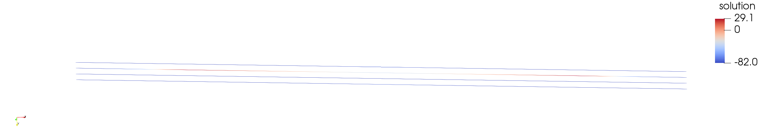
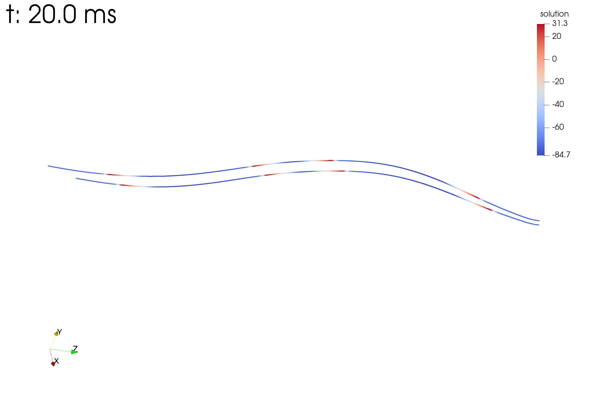
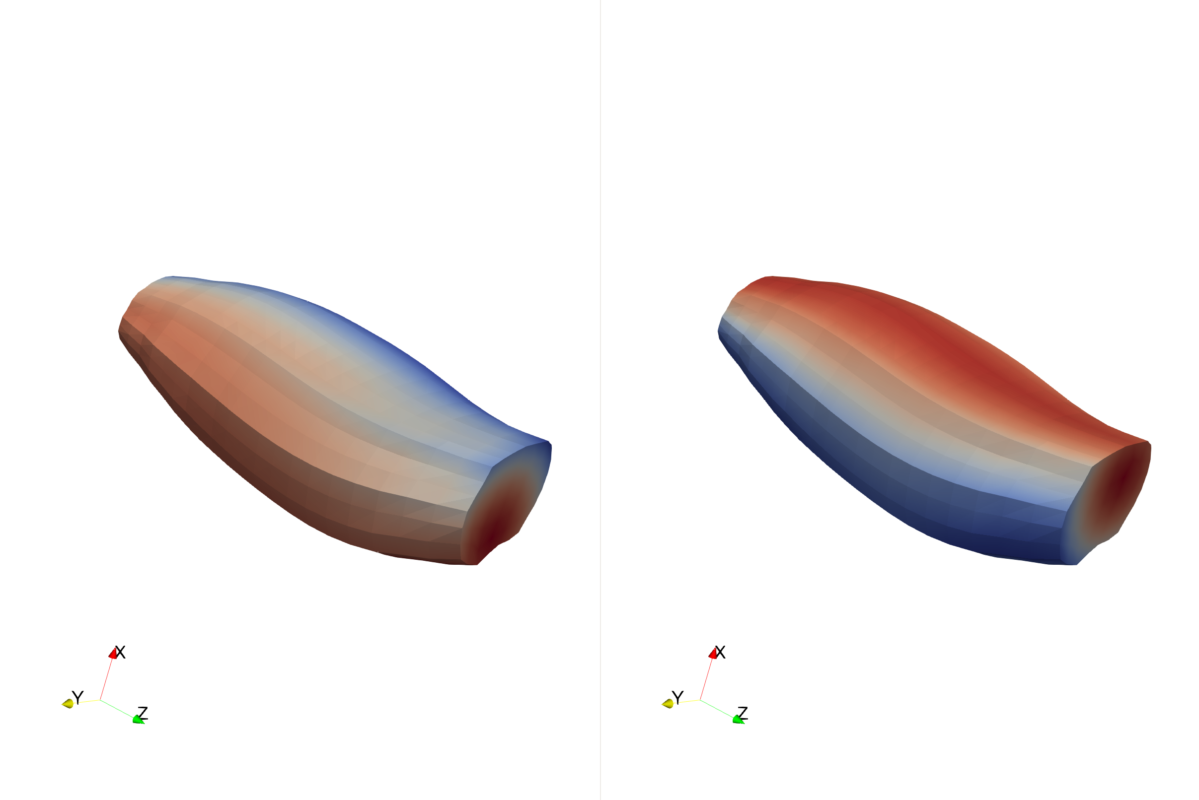
Fig. 59 The two fibers that are simulated in scenarios (1) and (2) at t=20.
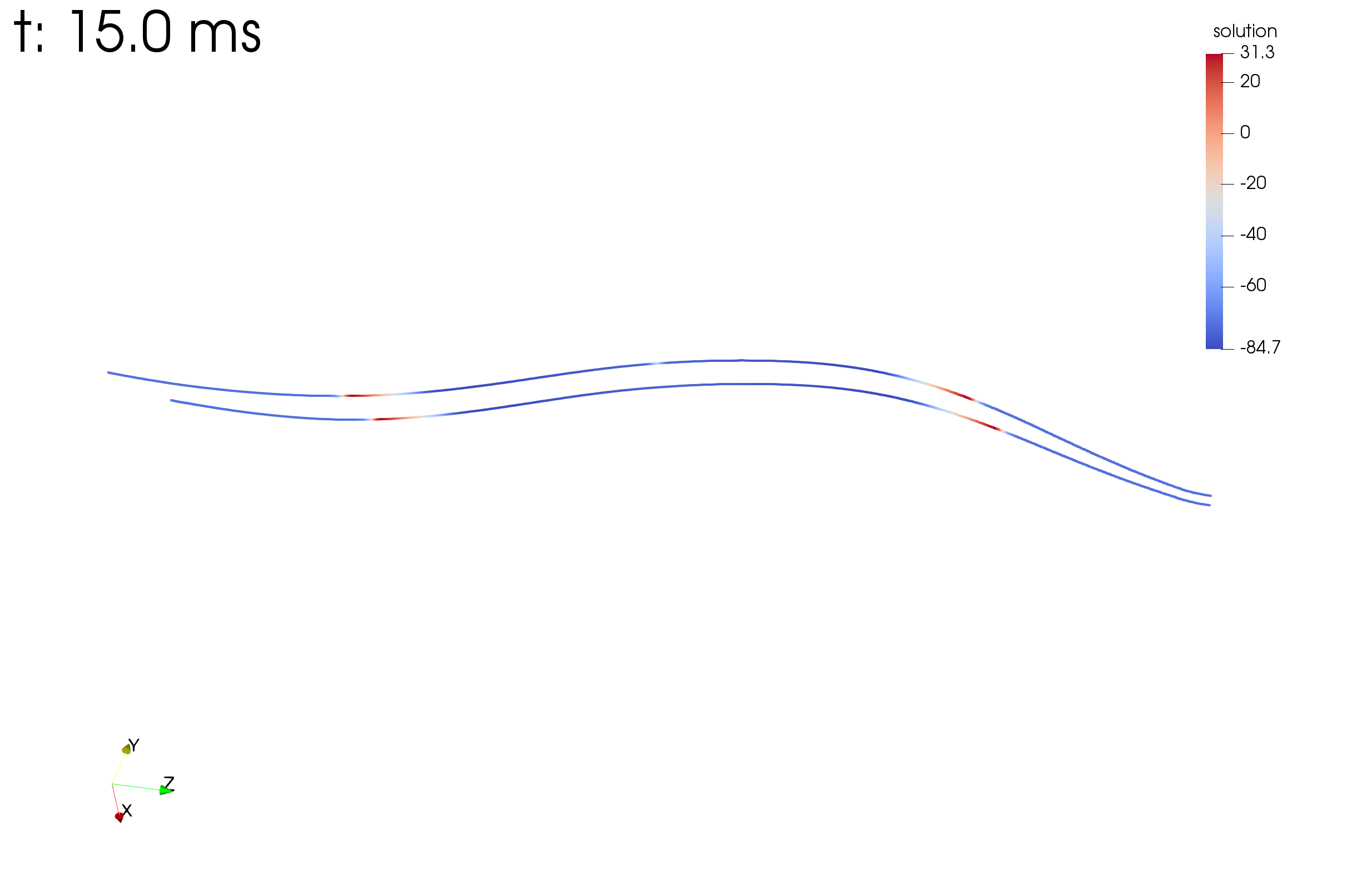
Fig. 60 The two fibers that are simulated in scenarios (1) and (2) at t=15.
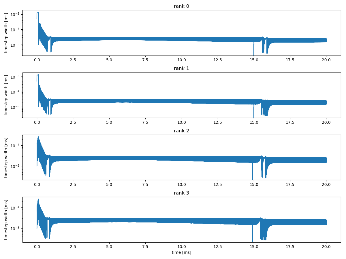
Fig. 61 Timestep widths during the simulation of scenario (1) on all ranks. It can be seen that the timestep width jumpes between values.
If a timestep width was fine, it is increased until it is too high, then it is reduced again. At \(t \approx 15\), two new action potentials start at the center, as can be seen in Fig. 60.
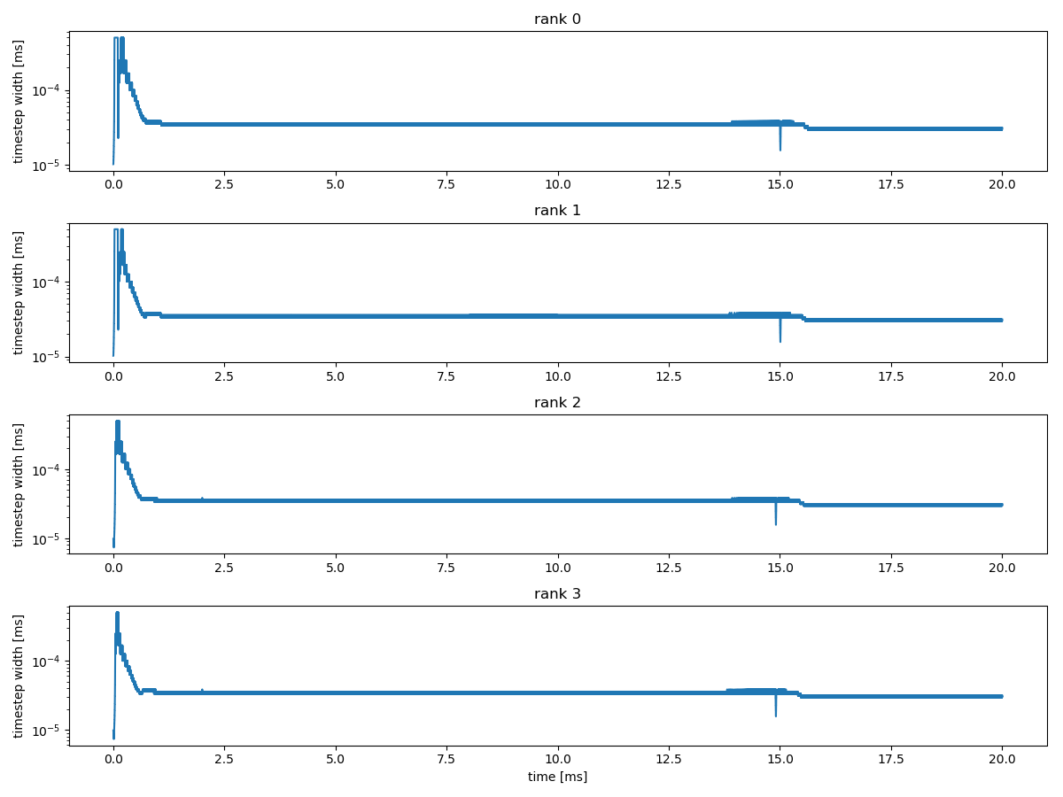
Fig. 62 Timestep widths during the simulation of scenario (2) with the modified adaptive Heun algorithm.
The results of two different strategies for adapting the time step width can be seen in Fig. 61 and Fig. 62.
The total runtimes of 20ms of simulation times are 7:13.14 min (regular) and 3:51.5 min (modified) and 2:27.52 min (FastMonodomainSolver) and 4s (FastMonodomainSolver with higher timestep widths that are still converging).
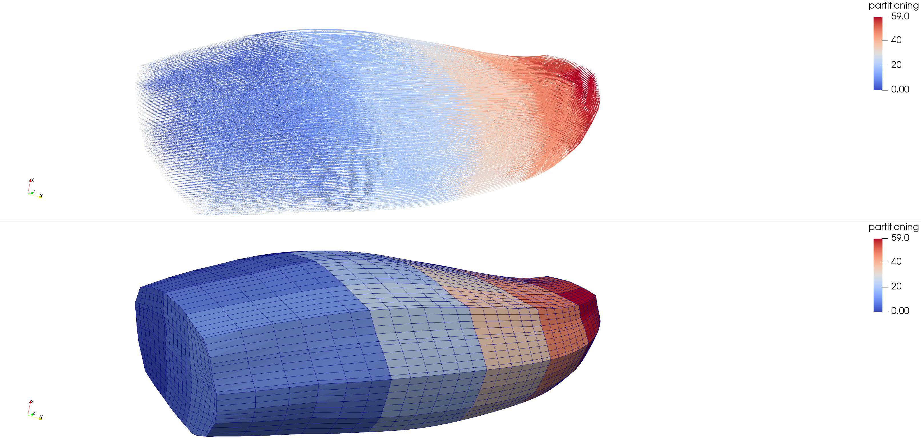
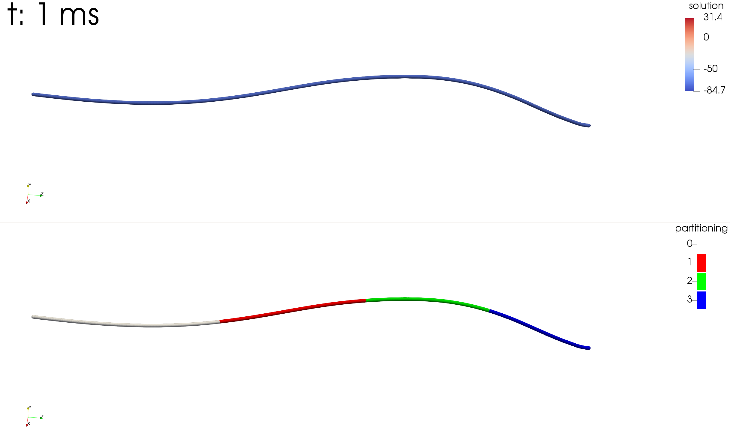
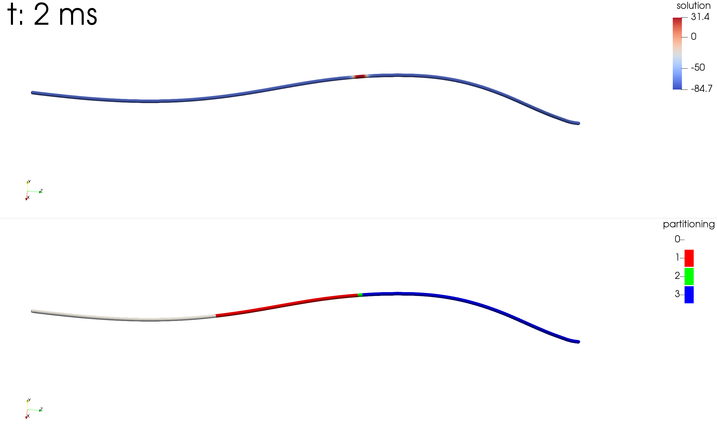
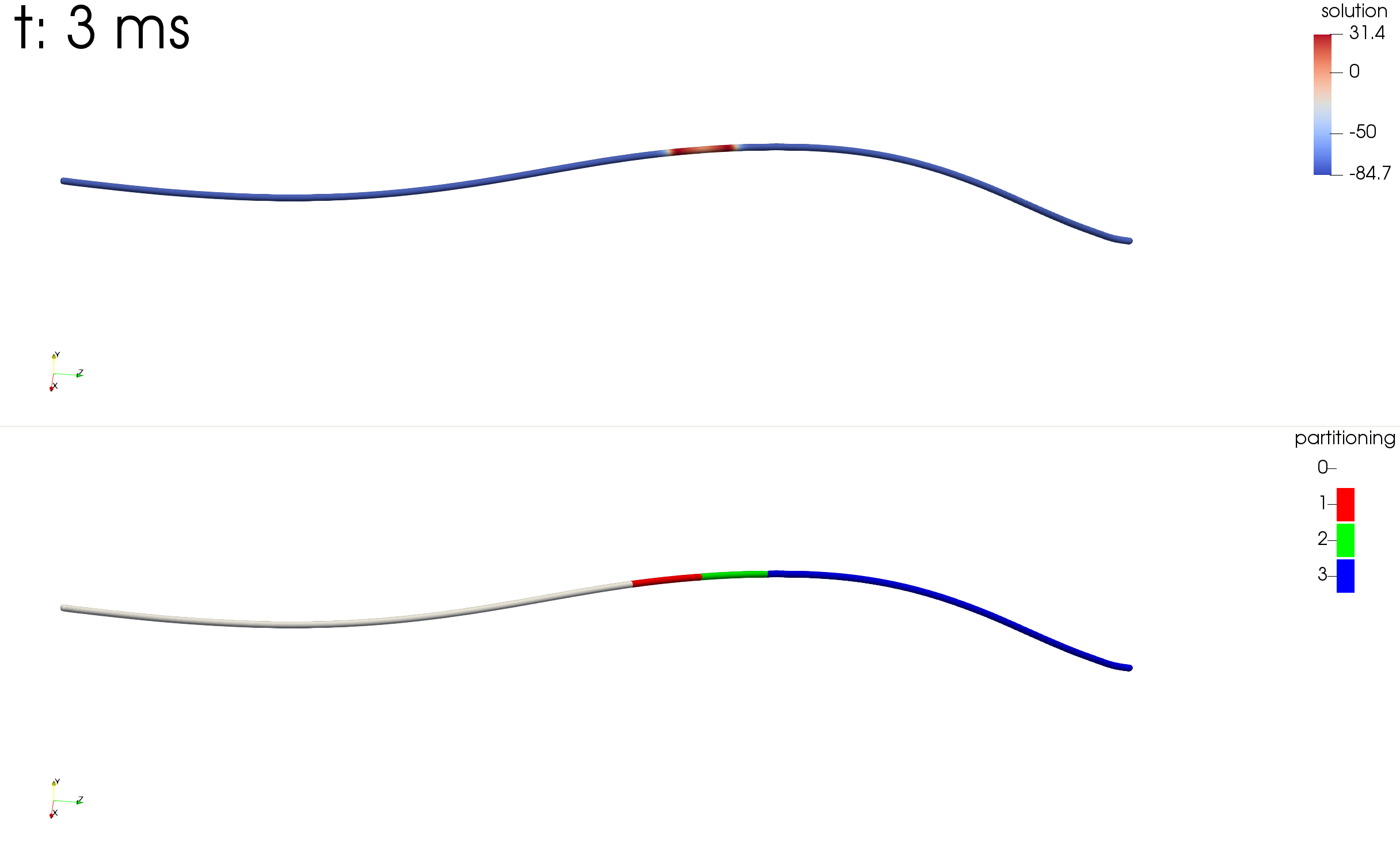
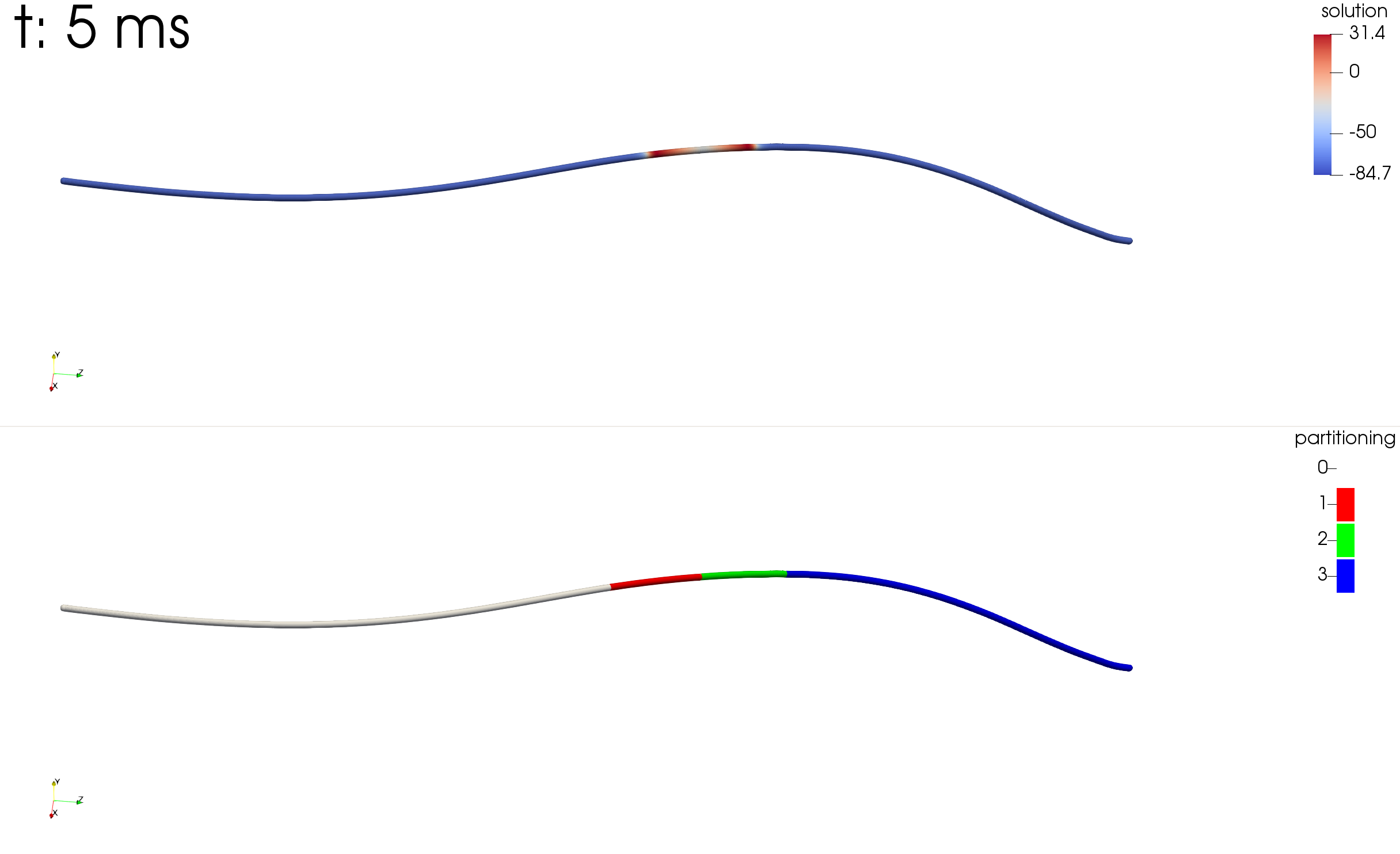
The second program uses dynamic load balancing and changes the domain on a single fiber that is computed by a process.
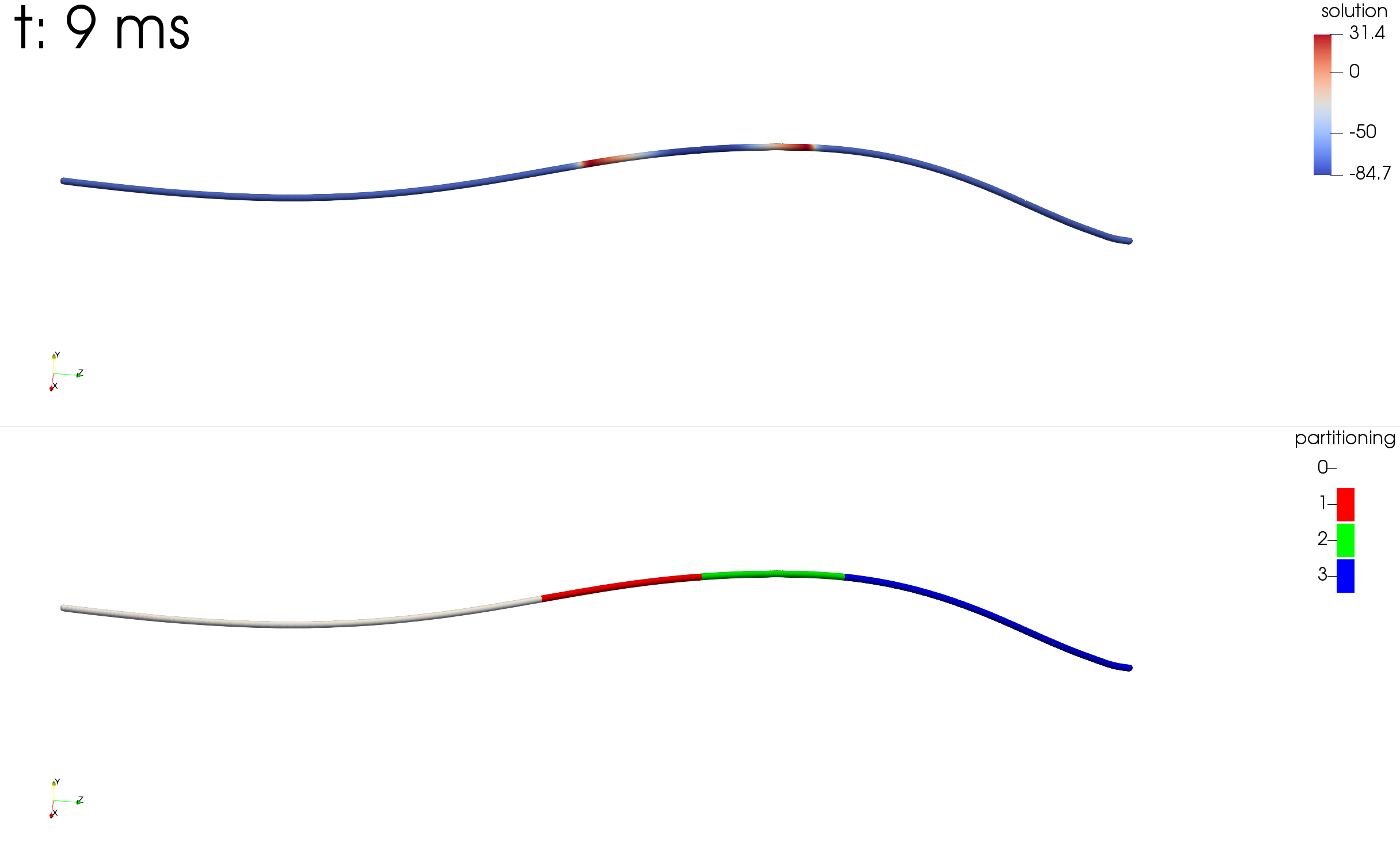
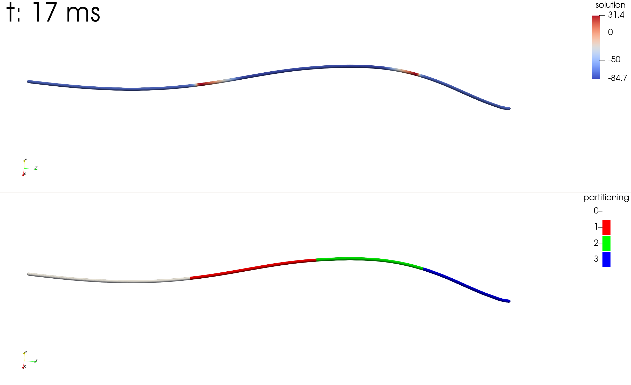
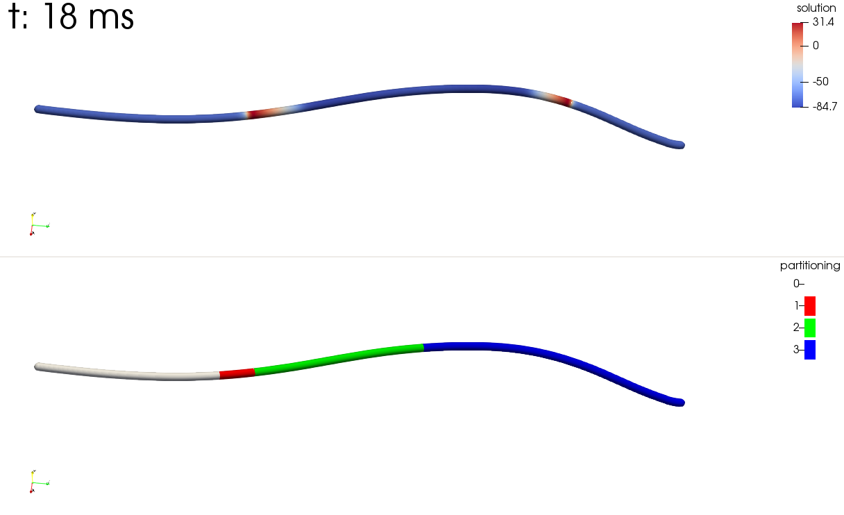
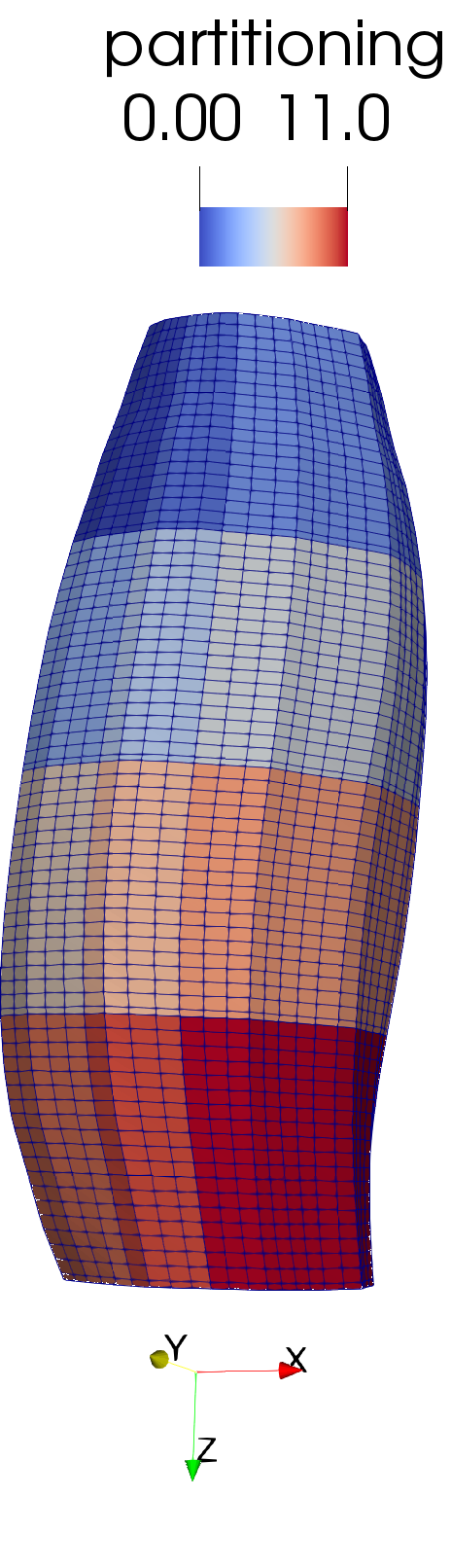
The results can be seen in the following images. Top shows the solution, bottom shows the rank partitioning to 4 ranks. In locations of the stimulus, a higher time step width is used, therefore the overall domain to be computed is smaller.
Scenario (1) uses the hodgkin-huxley_razumova subcellular model, which is just Hodgkin-Huxley for action potentials and Razumove for the active stress computation. This allows a fast computation.
Scenario (2) uses the Shorten model.
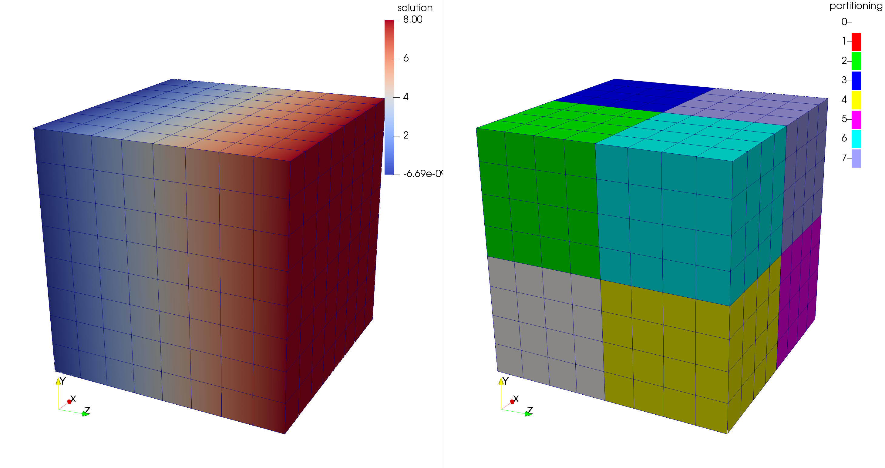
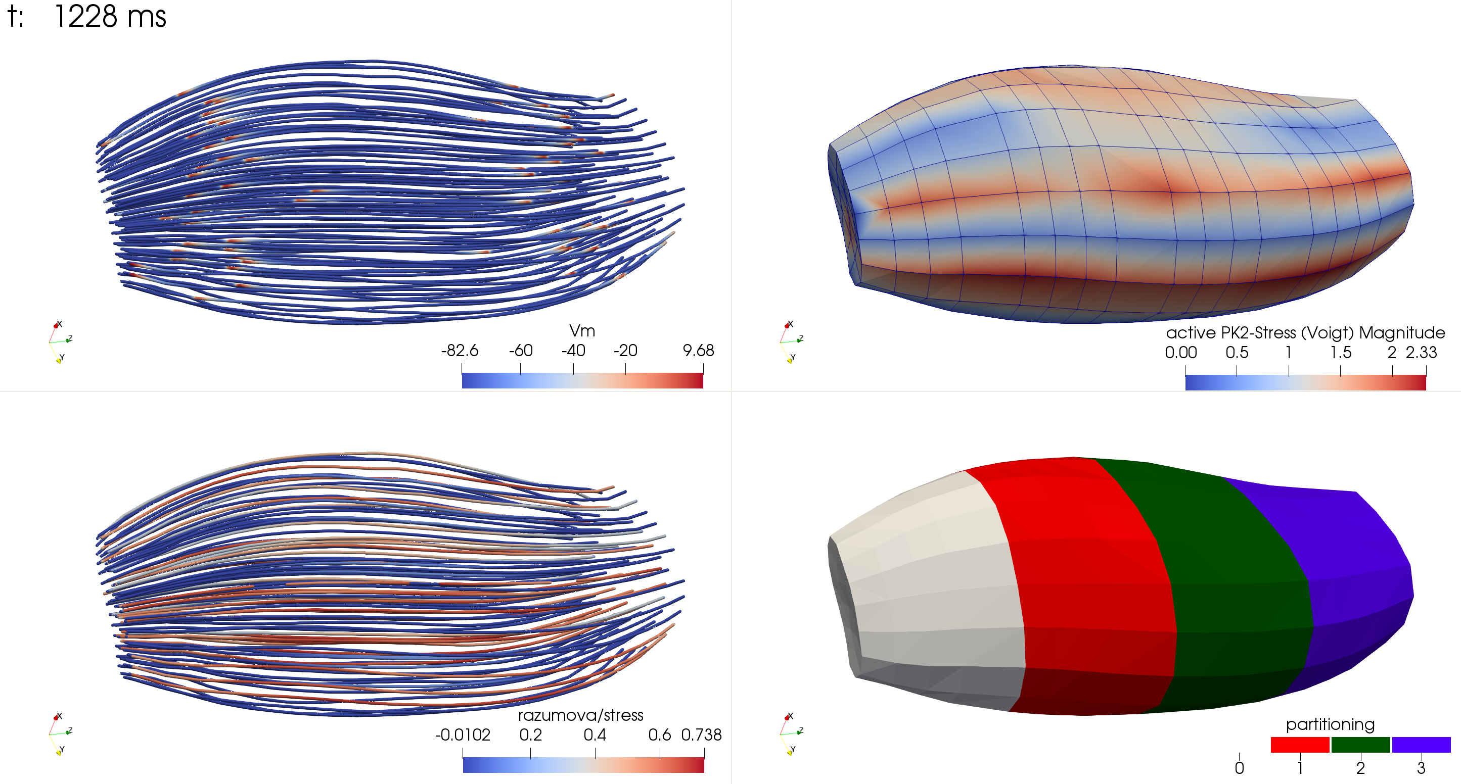
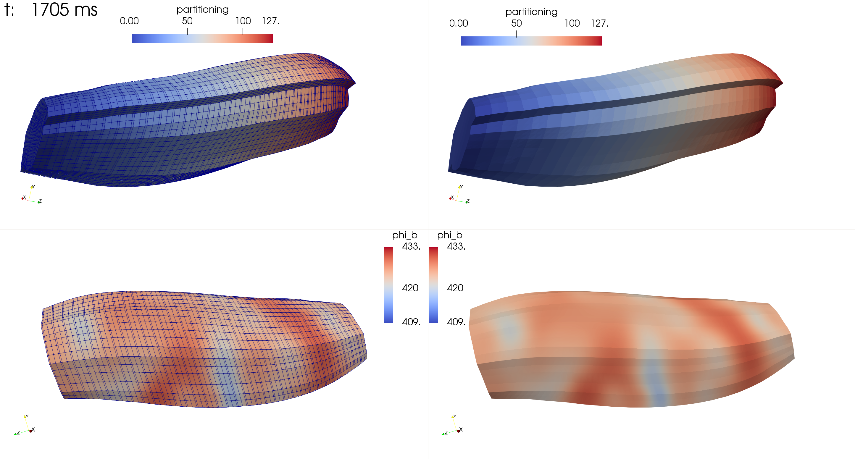
Fig. 63 Visualization of scenario (1), top left: Vm, top right: homogenized gamma, bottom left: active stress, bottom right: partitioning.
This is a video of the simulation of scenario (1), with end time of 4 seconds.
This example uses precice to couple the muscle and tendon solvers.
The muscle material is incompressible hyperelastic. The tendon material is compressible hyperelastic. Either an isotropic linear Saint-Venant Kirchhoff material or the anisotropic tendon material is used.
There are different scenarios with different material models and different coupling schemes.
Precice needs to be enabled in the user-variables.scons.py file. The example
cd$OPENDIHU_HOME/examples/electrophysiology/fibers/fibers_contraction/with_tendons_precice/only_tendon_static
.run_force.sh# run study
./tendon_precice_quasistaticsettings_only_tendon.py--fiber_file=../meshes/tendon_box.bin--force=1000# run a single simulation
Only Tendon
This settings file is to test and debug the tendon material. A box that is fixed on the right and pulled to the left is simulated. The data from this paper can be reproduced, but adjusting the material parameters for all variants.
The geometry can be created by the script create_cuboid_meshes.sh (you have to read this file and make adjustments to the mesh sizes etc.). The precice adapter is disabled.
Run as follows, adjust the geometry file as needed.
cd$OPENDIHU_HOME/examples/electrophysiology/fibers/fibers_contraction/with_tendons_precice/only_tendon_static
.run_force.sh# run study
./tendon_precice_quasistaticsettings_only_tendon.py--fiber_file=../meshes/tendon_box.bin--force=1000# run a single simulation
Fig. 64 A result of the tensile test of a cuboid tendon.
There are other examples where only the tendon (with real geometry or as a box) is computed. Try all directories that start with only_tendon_.
Explicit Neumann-Dirichlet
Scenario with explicit Neumann-Dirichlet coupling. Only one tendon (the bottom tendon) plus the muscle volume is considered here.
The muscle solver sends displacements and velocities at the coupling surface to the tendon solver, where these values are set as Dirichlet boundary conditions.
The tendon solver sends traction vectors at the coupling surface to the muscle solver where they act as Neumann boundary conditions.
Run the muscle and tendon solvers in two separate terminals. They will communicate over precice.
The precice settings file is precice_config_muscle_neumann_tendon_dirichlet.xml.
This does not converge, after some timesteps it will fail. This is because of the explicit timestepping and the choice that the muscle has the Neumann boundary conditions and the tendon has the Dirichlet boundary conditions.
Explicit Dirichlet-Neumann
Scenario with explicit Neumann-Dirichlet coupling, the other way round.
The muscle solver sends traction vectors at the coupling surface to the tendon solver where they act as Neumann boundary conditions.
The tendon solver sends displacements and velocities at the coupling surface to the muscle solver, where these values are set as Dirichlet boundary conditions.
Run the muscle and tendon solvers in two separate terminals. They will communicate over precice.
The precice settings file is precice_config_muscle_dirichlet_tendon_neumann.xml.
This scenario converges and works better than Explicit Neumann-Dirichlet.
Note that there is a variant of this scenario in dirichlet_neumann_linear which uses a linear hyperelastic material for the tendon.
Implicit Dirichlet-Neumann
This is the same as explicit Dirichlet-Neumann scenario but this time with implicit coupling in precice.
The precice settings file is precice_config_muscle_dirichlet_tendon_neumann.xml. This scenario also works.
Linear Implicit Dirichlet-Neumann
This is the same as Implicit Dirichlet-Neumann scenario except that it uses a linear Saint-Venant Kirchhoff material for the tendon instead of the nonlinear Tendon material. Note that the tendon is still geometrically nonlinear and therefore needs to be solved by a Newton scheme.
This scenario is a bit faster than Implicit Dirichlet-Neumann because of the tendon solver. It also has better convergence properties.
Multiple Tendons
This example simulates the biceps muscle with both tendons. It uses the Saint-Venant-Kirchhoff material for the tendons. The top tendons are represented by two separate meshes. In total, there are 4 coupling participants that are implicitely coupled with precice: three tendons, one muscle.
The multidomain equations are the 3D homogenized formulation of electrophysiology that replace the Monodomain Equation and the need for fibers. The 3D meshes are created from the same files that also contain the fiber information.
This means we still have fibers in the geometry description. Also the relative factors \(f_r\) are created as Gaussians with their center around particular fibers.
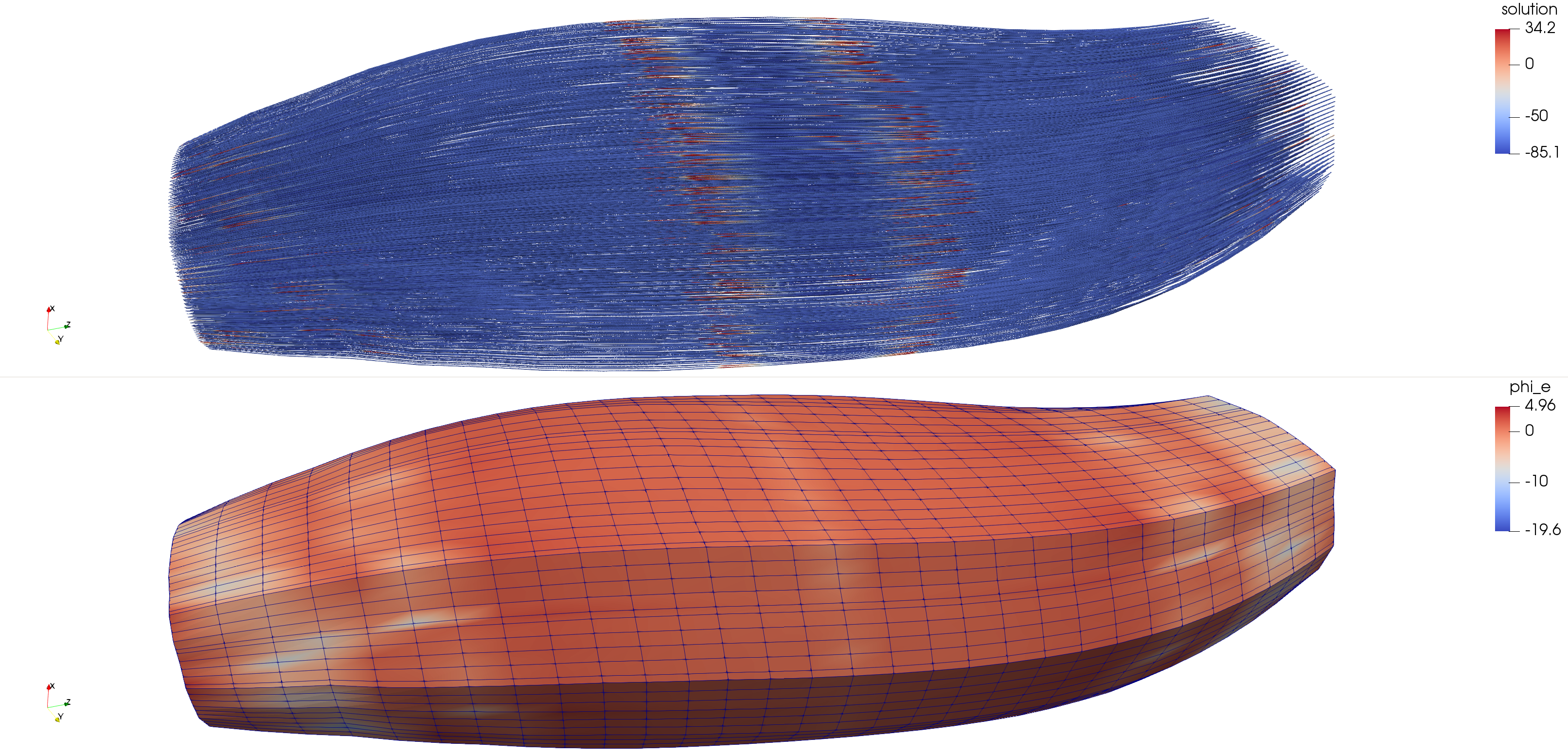
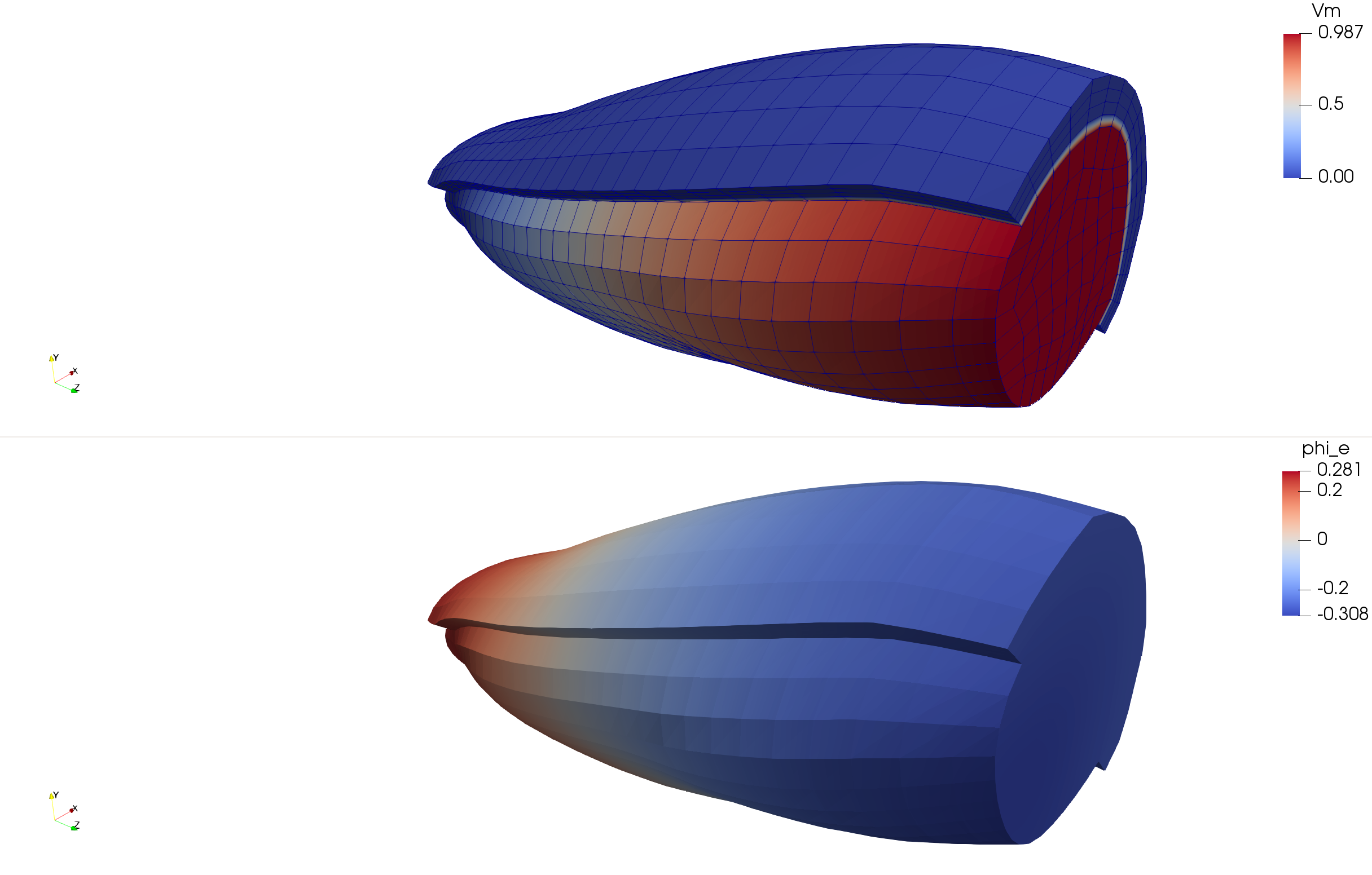
This example uses the StaticBidomainSolver and connects it to PrescribedValues. This allows to work with the Bidomain problem without any fibers or electrophysiology attached. Static Bidomain is listed under Multidomain because it is a specialization of the Multidomain Equations.
Examples that use the StaticBidomainSolver and electrophysiology using muscle fibers are fibers_emg and fibers_fat_emg.
Fig. 66 Models that are used in the static_bidomain example.
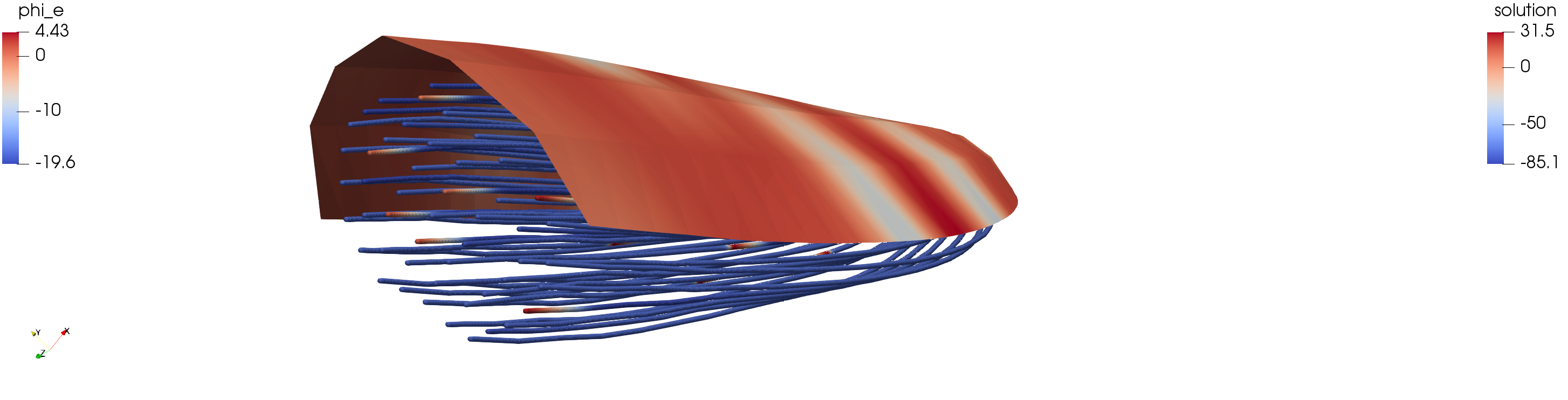
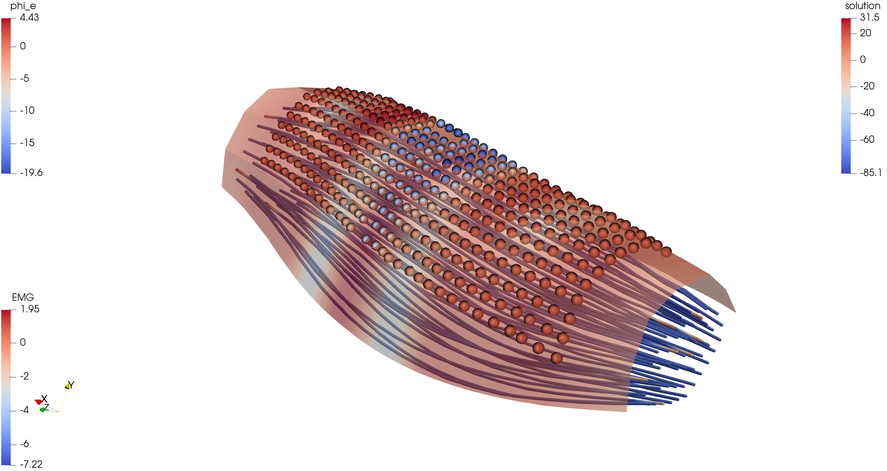
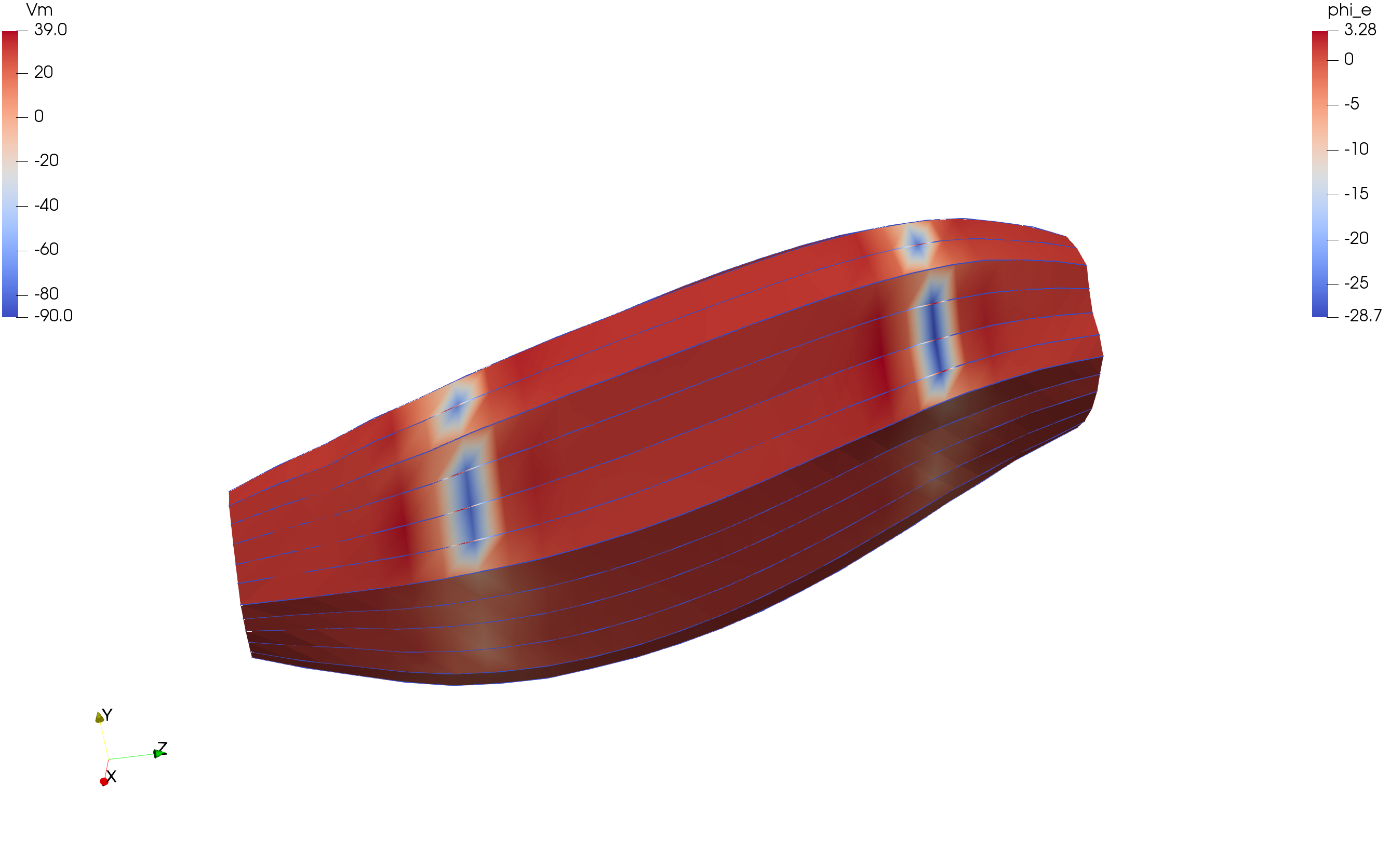
Fig. 67 Top image: prescribed trans-membrane potential, \(V_m\). The two meshes can be seen: the muscle belly (red) and the fat layer (blue) on top.
Bottom image: value of the extracellular potential, \(\phi_e\). A “wave” moves along the muscle because of the prescribed values of \(V_m\) given by the sine function.
Fig. 69 The relative factors, \(f_r^k\) for two compartments, \(k=1,2\).
Care must be taken to use exact solvers and low tolerances, as well as a high spatial resolution. Otherwise the stimuli will reflect at the boundaries of the muscle which is not physical.
This is the full Multidomain model also including a fat domain.
Fig. 70 Models that are used in the multidomain_with_fat example.
cd$OPENDIHU_HOME/examples/electrophysiology/multidomain/multidomain_with_fat
mkorn&&sr# buildcdbuild_release
mpirun-n12./multidomain_with_fat../settings_multidomain_with_fat.pyneon.py# short runtime
mpirun-n12./multidomain_with_fat../settings_multidomain_with_fat.pyramp_emg.py# longer
mpirun-n128./multidomain_with_fat../settings_multidomain_with_fat.pyramp_emg.py--n_subdomains4132
Instead of 12 processes, any other number can be used.
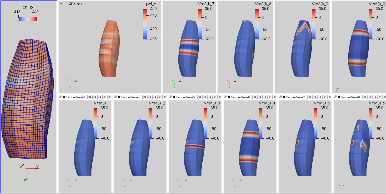
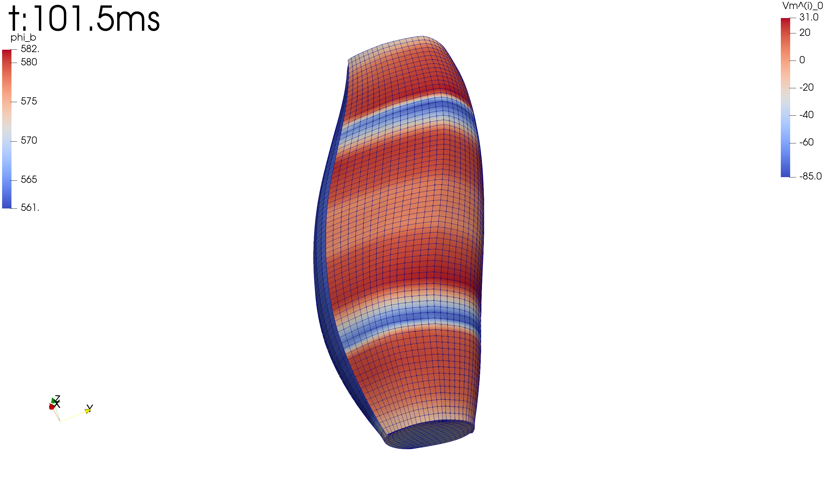
EMG on the surface, at t = 1.406 s. Also the fine resolution can be seen
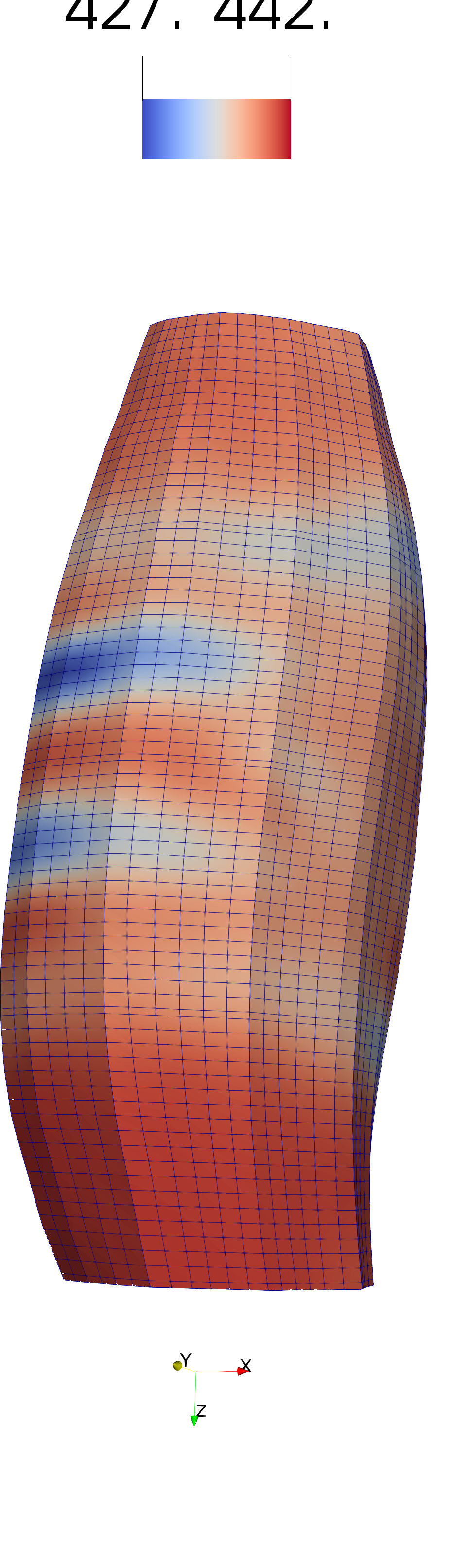
Fig. 71 View of \(V_m\) in all 10 compartments (small images at the right), the resulting potential in the body domain, \(\phi_b\) (top center), and the surface EMG (left, big)
Fig. 73 This is the scenario with 128 processes, top: partitioning, each color corresponds to one rank. Bottom: EMG signal, it can be seen that this is very smooth, because of the high spatial resolution.
This is the Multidomain model with fat combined with muscle contraction.
Fig. 74 Models that are used in the multidomain_contraction example.
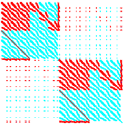
Fig. 75 The non-zero structure of the material Jacobian of the nonlinear problem, use options -mat_view draw -draw_pause 3 to display this structure.
Example with 3 x 3 x 10 = 90 global quadratic elements in the muscle domain and 6 x 1 x 10 = 60 elements in the fat domain, in total 150.
Fig. 77 Models that are used in the only_neurons_hodgkin_huxley example.
This example implements muscle spindles, Golgi tendon organs, interneurons and motor neurons. All sensors and the interneurons use the Hodgkin-Huxley CellML model. The motoneuron uses the MN_Cisi_Kohn_2008 model.
The architecture is shown in Fig. 78.
Fig. 78 Schematic of the architecture of sensor organs and neurons that is implemented.
Compile and run the example like the following, then call the python plotting script.
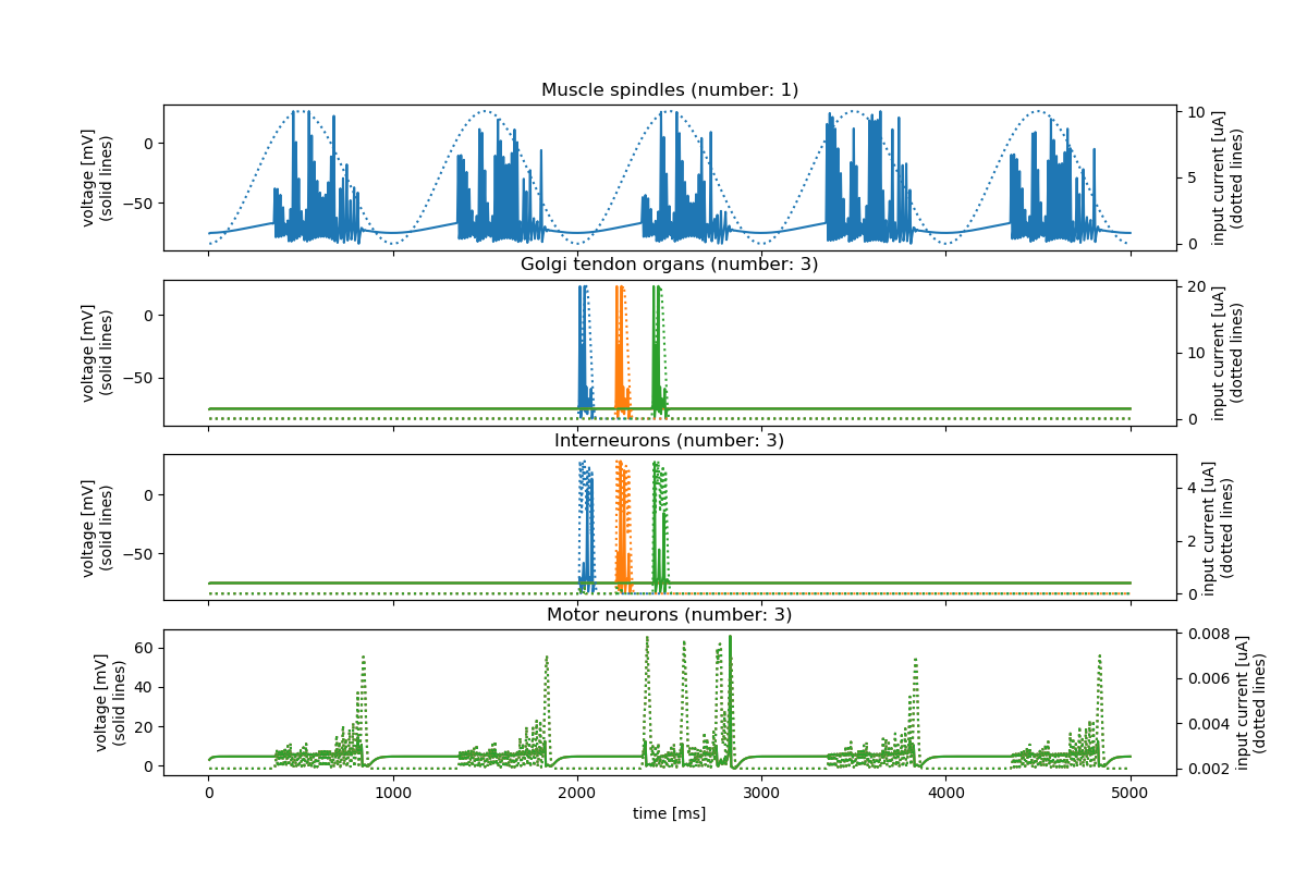
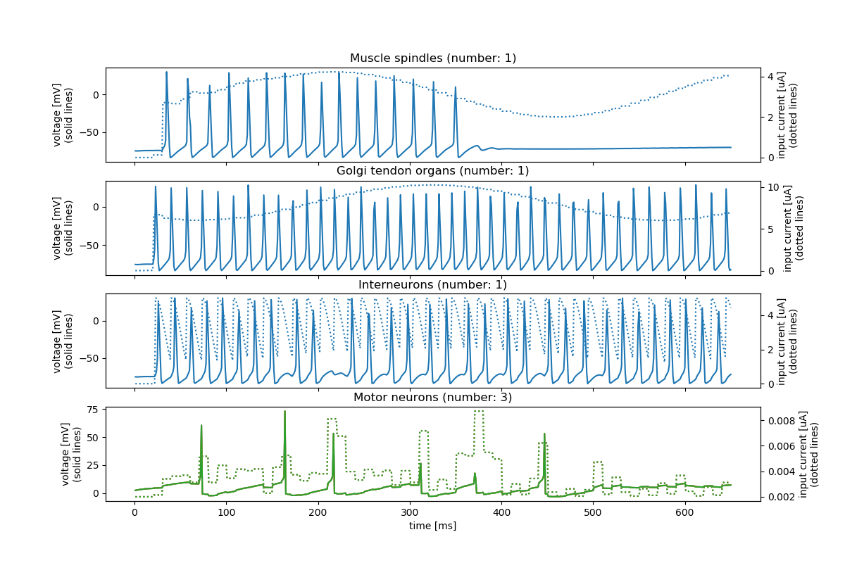
Fig. 79 Plot window of the scenario. In the top plot, the muscle spindle input (dotted lines) and output (solid lines) are shown. The input is prescribed by a \(\sin^2(t)\) function.
The second and third plots show the Golgi tendon organs and the interneurons, again with inputs (dotted lines) and outputs (solid lines). There are three instances of each of them.
The input to the motor neurons is shown in the bottom plot by the dotted lines. It is the sum of the scaled outputs of Interneurons and Muscle spindles, with a time delay from the interneurons.
The output of the motor neurons are the solid lines at the bottom.
Logically the same as only_neurons_hodgkin_huxley. The structure of the c++ main file is different. It does not use the Control::MultipleCoupling scheme, instead is uses 4 nested Control::Coupling schemes which is very confusing.
This example is kept here, because it works and for learning purposes, to demonstrate how to not use Control::MultipleCoupling.
You can compare the solver_structure.txt files of the examples only_neurons_hodgkin_huxley and only_neurons_hierarchical_structure.
This example combines the sensors and neurons with the elasticity solver. The architecture in Fig. 78 also holds for this example.
The active stress \(\gamma\) in the 3D domain is prescribed by a \(sin\) function. The 3D mechanics is computed with the muscle material. The muscle spindles and Golgi tendon organs get their values from the deforming 3D domain.
All sensors and the interneurons use the Hodgkin-Huxley CellML model. The motoneuron uses the MN_Cisi_Kohn_2008 model.